
下载掌阅APP,畅读海量书库
立即打开


 轨线的拓扑分类
 Wtthelliptic Solution which Contact Both Axes
Abstract : In this paper we have studied the phase portrait of the kolmogorov cubic system E 3 2 with an elliptic solution which contacts both the axes. We have proved that there are altogether eight types of the topological structure of this system. Besides, if we consider this system as a mathematical model, among these eight types of topological structure of the system, only one type has practical significance.
Article [1] discussed that the kolmogorov cubic system with an elliptic solution can only possibly have periodic region, but can not have any limit cycles. Article [2]discussed that the kolmogorov cubic system with an elliptic solution which contacts both the axes can possibly have limit cycles. Article [2] only made this system with a weak focus by means of an example with a practical system and proved the existence of the limit cycles by using the Hopf bifurcation.
But about the topological structure of the tvajectories of this type of system, we know nothing at all. Actually for the kolmogorov cubic system which connects closely with practice, the more important thing is to study the phase portrait of this system. As it is very difficult to study the phase portrait of general kolmogorov cubic system,according to the principle from particularity to generality, we begin to discuss only the phase portrait of the particular kolmogorov cubic as in the following.
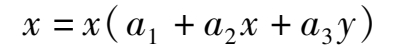

We will prove that there are altogether eight types of the topological structure of these systems. After a scale transformation, the elliptic equation contacting with two axes changes to the simpler form.

Here | α | < 1. When α = 0, the ellipse becomes a circle. It is located in the first quadrant.
Theorem
1
The sufficient and necessary condition of the existence of elliptic solution (1)(
α
≠0) of the system
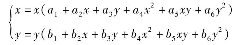
 is that the system can be expressed in the following form.
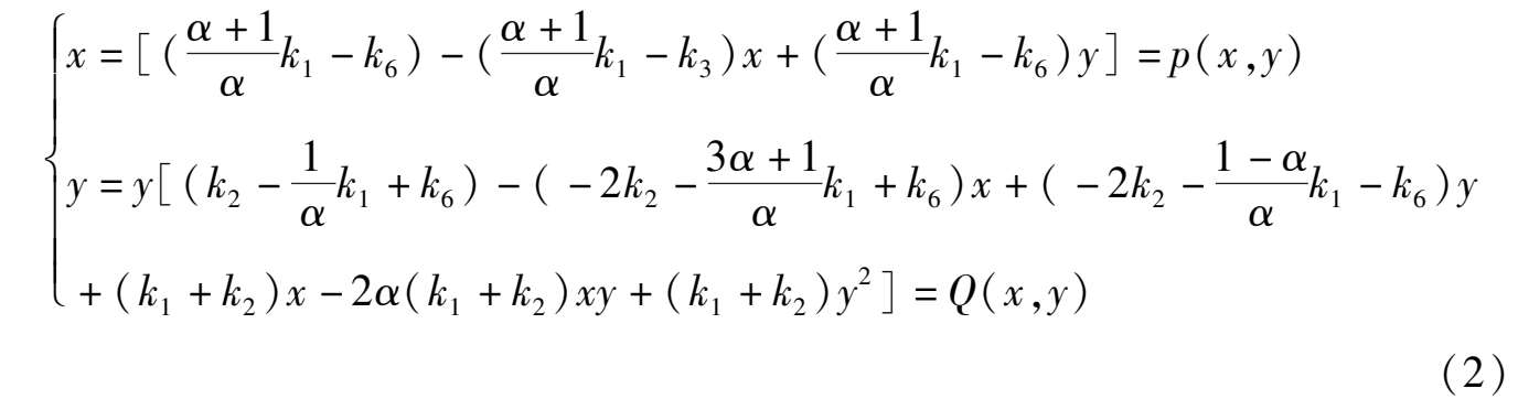
Proof Form article [2] we know that the sufficient and necessary condition of the existence of elliptic solution (1) of system.
is that the system can be expressed in the following form.
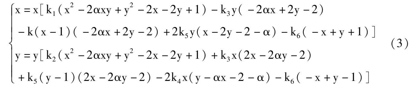
Substitute to system (3),we obtain system (2) immediately.
We can suppose k 1 + k 2 ≠0. If k 1 + k 2 = 0, then system (2) will degenerate into a quadratic system. If k 1 + k 2 > 0,by a transformation t →- t ,it can be changed to k 1 + k 2 < 0. Hence we can suppose k 1 + k 2 < 0 in system (2).
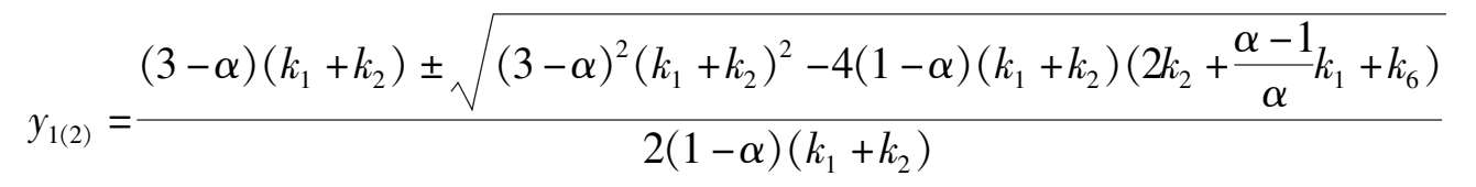
Corollary 1 System (2) has not more than six finite singularities, their coordinates are
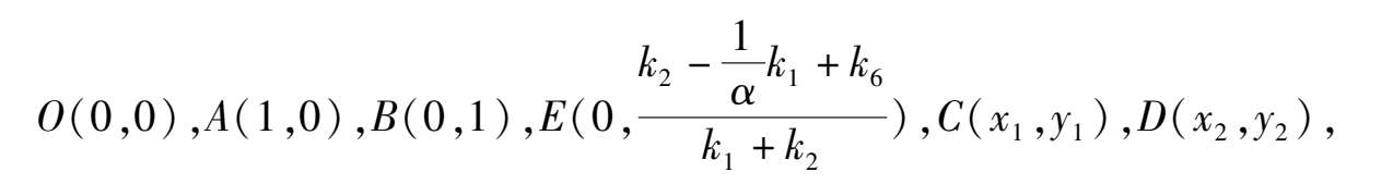
here
The proof is omitted.
Corollary
2
System (2) has two infinite singularities. Their coordinates are P(1,0,0). S(0,1,0),S(0,1,0)must be an unstable node. As for the P(1,0,0): if
 k
1
-
k
6
< 0,then the P(1,0,0) is a (right stable) node (left) saddle point; if
k
1
-
k
6
< 0,then the P(1,0,0) is a (right stable) node (left) saddle point; if
 k
1
-
k
6
> 0,then the P(1,0,0) is a (right) saddle (left stable) node.
k
1
-
k
6
> 0,then the P(1,0,0) is a (right) saddle (left stable) node.
Proof
After a transformation x =
 ,y =
,y =
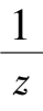
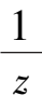
 for system (2),we obtain
If use the transformation x =
 ,y =
,y =
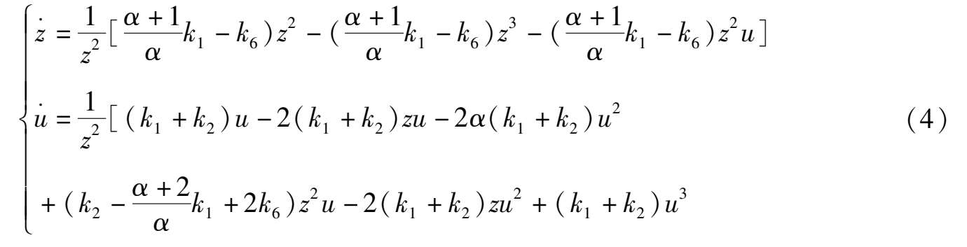
 for system (2),we obtain
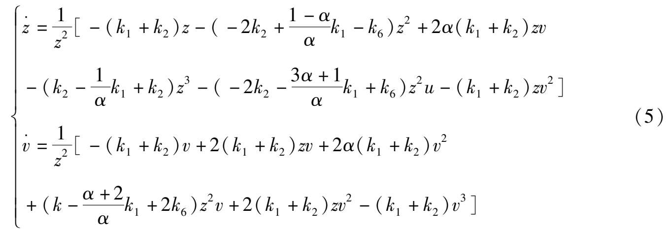
Because α 2 -1 < 0, system (2) has only two infinite singularities P (1,0,0) and S (0,1,0). Observing system (4) and (5),we can know at once that the properties of P and S as in Corollary 2 are correct.
In order to study the location and properties of finite singularities, we discuss the four different conditions separately.
(1)Point E is located at Y axis and above the B(1,0),which is
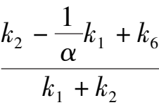 >1 ,
>1 ,
namely
k
6
-
 k
1
< 0.
k
1
< 0.
Corollary
3
Suppose
k
1
+
k
2
< 0,
k
6
-
 k
1
< 0, Again
k
1
< 0, Again
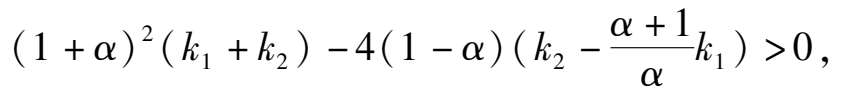
1)if
Δ
= (1 +
α
)
2
(
k
1
+
k
2
)
2
-4(1-
α
)(
k
1
+
k
2
)(
k
6
-
 k
1
)> 0,namely
k
1
)> 0,namely
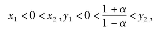
then the phase portrait of system (2) is indicated in Fig. 1(1);
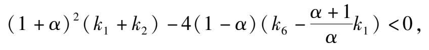
2) if Δ < 0,namely
then the phase portrait of system (2) is Fig. 1(2);
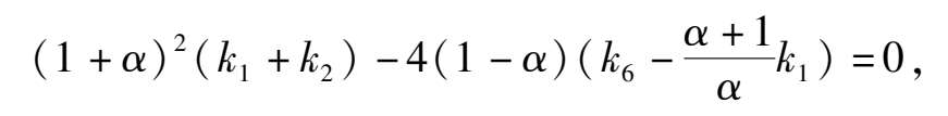
3) if Δ < 0,namely
then the phase portrait of system (2) is Fig. 1(3).
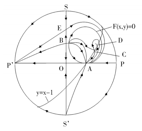
(1)
(2)
(3)
(4)
Fig. 1.
Proof
We had known that E is located at Y axis, and above B(1,0). We will consider the location about C(
x
1
,
y
1
) and D(
x
2
,
y
2
). When
k
6
-
 k
1
< 0, because 4(1-
α
)(
k
1
+
k
2
)(
k
6
-
k
1
< 0, because 4(1-
α
)(
k
1
+
k
2
)(
k
6
-
 k
1
)> 0
y
2
>
y
1
> 0, namely C and D which locate on
y
=
x
-1,they are in the first quadrant. Further we deduce that 0 <
y
1
<
y
2
<
k
1
)> 0
y
2
>
y
1
> 0, namely C and D which locate on
y
=
x
-1,they are in the first quadrant. Further we deduce that 0 <
y
1
<
y
2
<
 ,where
 is a ordinate of the intersection of the straight line
y
=
x
-1 and ellipse(1),so C and D are located inside ellipse(1) and the C is located between A and D.
is a ordinate of the intersection of the straight line
y
=
x
-1 and ellipse(1),so C and D are located inside ellipse(1) and the C is located between A and D.
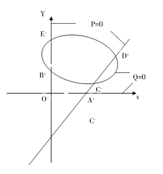
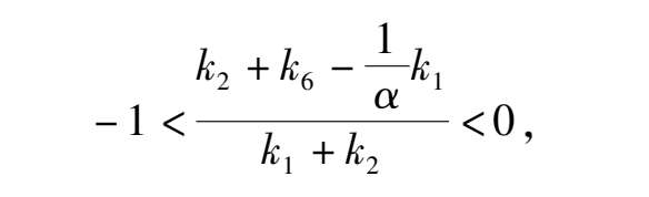
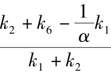
We discuss the properties of these finite singularities. Fram system(2),we know that the P(x,y) = 0 are two straight lines x = 0 and y = x -1;while the Q(x,y) = 0 is a straight line y = 0 and an ellipse. When Δ > 0, the ellipse pass through these four singularities B. C. D. E. as shown in figure1(4). According to article [3],we know that the index of O. E. C. is-1,and the index of A. B. D. is + 1. It is easy to know that they are elementary singularities, so the Fig. 1(1) is correct, except that the stability of the point D remains to be distinguished.
A s fo r t h e p o i n t D ,w e h a v e (
P
x
+
Q
y
)
D
=
 k
1
-
k
6
> 0, Therefore D i s a n unstable focus (node) point. When Δ = 0,the point C and D coincide and become one point. Now, for the system (2) we obtain the matrix.
k
1
-
k
6
> 0, Therefore D i s a n unstable focus (node) point. When Δ = 0,the point C and D coincide and become one point. Now, for the system (2) we obtain the matrix.
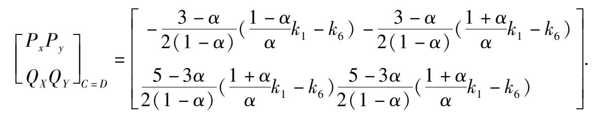
Because these two column elements are in proportion, and(
P
x
+
Q
y
)
C
= D=
 k
1
-
k
6
> 0, therefore C and Dcoincide and become a saddle(unstable) node, as shown in figue1(2). When Δ < 0,C and D disappeared. Its phase portrait must be indicated by figue1 (3).
k
1
-
k
6
> 0, therefore C and Dcoincide and become a saddle(unstable) node, as shown in figue1(2). When Δ < 0,C and D disappeared. Its phase portrait must be indicated by figue1 (3).
Note the proof of Corollary 3. If we distinguish the property of every finite singularity. Through calculation, the result will be the same. But if we do so, there will be a large amount of calculation and a great length of space.
(2) Point E is located at Y axis and between B and O, that is 0 <
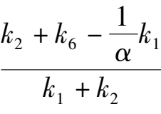 < 1, namely
k
2
+
k
2
-
< 1, namely
k
2
+
k
2
-
 k
< 0,and
k
6
-
k
< 0,and
k
6
-
 k
1
> 0.
k
1
> 0.
Corollary
4
Suppose
k
1
+
k
2
< ,
k
6
-
 k
1
> 0,
k
2
+
k
6
-
k
1
> 0,
k
2
+
k
6
-
 k
1
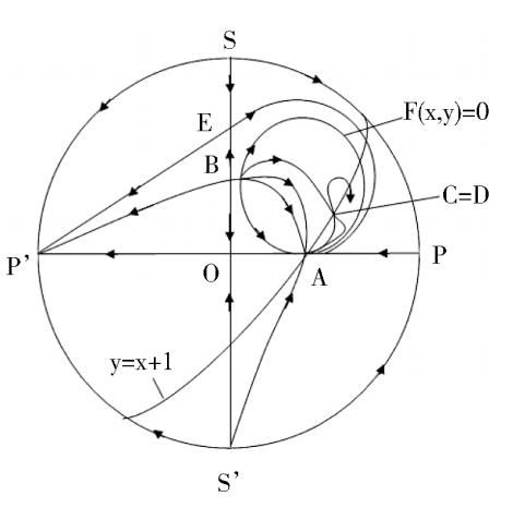
< 0 ,the phaseportrait of system (2) is indicated in Fig. 2 (1).
k
1
< 0 ,the phaseportrait of system (2) is indicated in Fig. 2 (1).
Proof
We had known that the E is located at y axis between B and O. As for the locating of C(
x
1
,
y
1
),D(
x
2
,
y
2
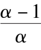
),because
k
6
+ 2
k
2
-
 k
1
=
k
6
+
k
2
-
k
1
=
k
6
+
k
2
-
 k
1
+ (
k
1
+
k
2
) < 0,we can deduce that 0 <
x
1
<
x
2
,
y
1
< 0
k
1
+ (
k
1
+
k
2
) < 0,we can deduce that 0 <
x
1
<
x
2
,
y
1
< 0
 <
y
2
easily, namely C is located in the fourth quadrant and D is located above the ellipse(1).As shown in Fig.2(2).
<
y
2
easily, namely C is located in the fourth quadrant and D is located above the ellipse(1).As shown in Fig.2(2).
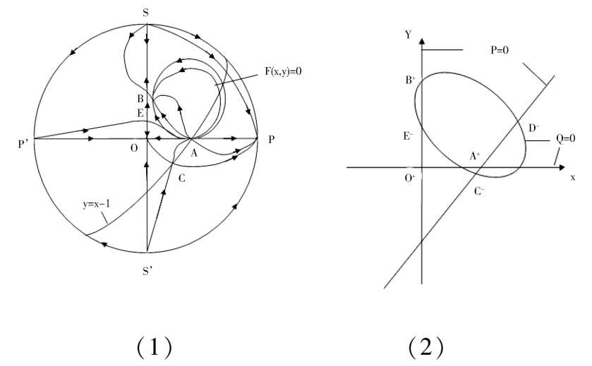
Fig. 2.
According to article [3],we know that Fig. 2(1) is exactly correct.
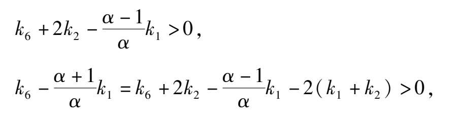
(3)Point E is located at negative y axis and above the straight line y = x-1, that is
namely
Corollary
5
Suppose
k
1
+
k
2
< 0,
k
6
+
k
2
-
 k
1
> 0,
k
6
+ 2
k
2
-
k
1
> 0,
k
6
+ 2
k
2
-
 k
1
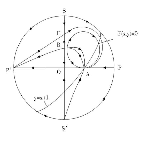
< 0,thephase portrait of system (2) is indicated in Fig. 3 (1).
k
1
< 0,thephase portrait of system (2) is indicated in Fig. 3 (1).
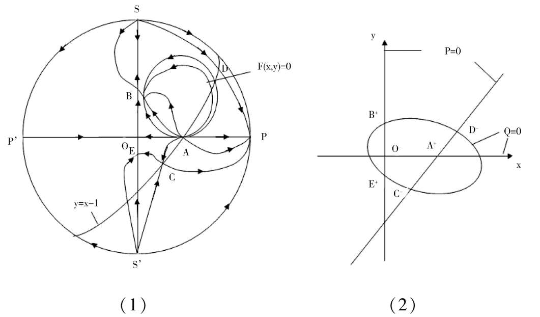
Fig. 3.
Proof We had known that E is located any axis and between 0 and straight line y= x-1. As for the location of C ( x 1 , y 1 ),D( x 2 , y 2 ), because

we can deduce that
x
1
> 0,
x
2
> 0,
y
1
< 0 <
 <
y
2
easily, so C is located in the fourth quadrant and the D is located above the ellipse (1),as shown in Fig. 3 (2).According to article [3],we know that Fig. 3(1) is exactly correct.
<
y
2
easily, so C is located in the fourth quadrant and the D is located above the ellipse (1),as shown in Fig. 3 (2).According to article [3],we know that Fig. 3(1) is exactly correct.
(4)Point E is located at negative y axis and below the straight line y = x-1,that is
 <-1, namely
k
6
+ 2
k
2
-
<-1, namely
k
6
+ 2
k
2
-
 k
1
> 0.
k
1
> 0.
Corollary
6
Suppose
k
1
+
k
2
< 0,
k
6
+ 2
k
2
-
 k
1
> 0, the phase portrait of system (2) is indelicate in Fig. 4(1).
k
1
> 0, the phase portrait of system (2) is indelicate in Fig. 4(1).
Proof We had known that E is located at negative y axis and below the straight line y = x-1.
As for the location of C( x 1 , y 1 ),D( x 2 , y 2 ), because
we can deduce that
so the C is located in the third quadrant and the D is located above the ellipse(1),as shown in Fig. 4 (2). According to article [3],we know that Fig. 4 (1 ) is exactly correct only the stability of C remains to be distinguished.
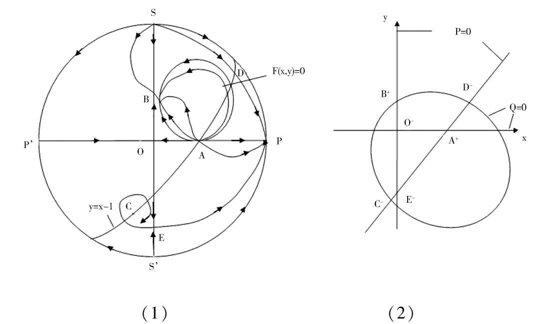
Fig. 4.
Since(
P
x
+
Q
y
) C =
 k
1
-
k
6
< 0, C is stable focus ( node).( If there have limit cycles surrounding the point C, the number of limit cycles must be even. But we estimate that it will not happen. ).
k
1
-
k
6
< 0, C is stable focus ( node).( If there have limit cycles surrounding the point C, the number of limit cycles must be even. But we estimate that it will not happen. ).
We go on with our work to study the following three cases:i)E coincides to B ( namely the condition
k
6
-
 k
1
= 0),ii) E coincides to D (namely the condition
k
6
+
k
2
-
k
1
= 0),ii) E coincides to D (namely the condition
k
6
+
k
2
-
 k
1
= 0),iii) E is located on straight y = x-1,for this moment E coincides to C(namely the condition
k
6
+ 2
k
2
+
k
1
= 0),iii) E is located on straight y = x-1,for this moment E coincides to C(namely the condition
k
6
+ 2
k
2
+
 k
1
= 0).
k
1
= 0).
Corollary
7
If
k
1
+
k
2
< 0,
k
6
-
 k
1
= 0, the system (2) degenerates into the case
k
1
= 0, the system (2) degenerates into the case
 = 0;I f
k
1
+
k
2
<0 ,
k
6
+
k
2
-
= 0;I f
k
1
+
k
2
<0 ,
k
6
+
k
2
-
 k
1
= 0, the phase portrait of system (2) is indicated by Fig. 5;If
k
1
+
k
2
< 0,
k
6
+
k
2
+
k
1
= 0, the phase portrait of system (2) is indicated by Fig. 5;If
k
1
+
k
2
< 0,
k
6
+
k
2
+
 k
1
= 0, the phase portrait of system(2) is indicated by Fig. 6.
k
1
= 0, the phase portrait of system(2) is indicated by Fig. 6.
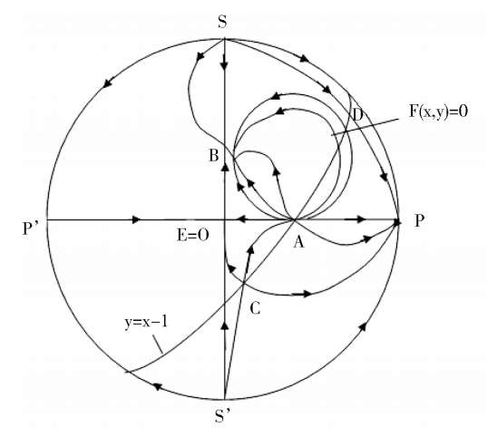
Fig. 5.
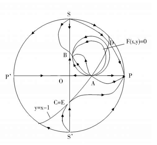
Fig. 6.
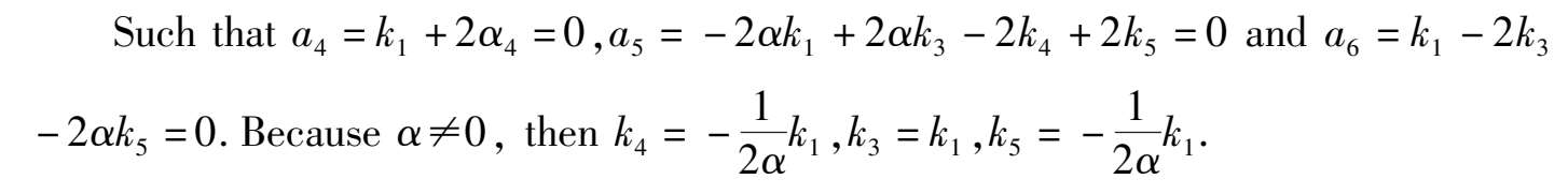
Finally, we will have to discuss continuously. When α = 0, then equation (1) change to a circle

The corresponding system (2) will change to the system
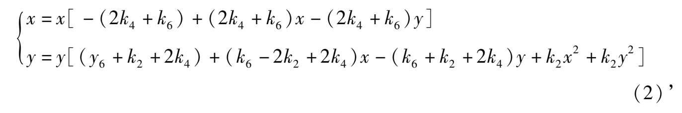
Without loss of generality, we can let k 2 < 0.(If = 0,system(2)’ can degenerate to a quadric system).
Corresponding to system (2),we have some corollaries of system(2)’ as in the following.
Corollary
1
’ System (2 )’ has not more than six finite singularities. Their coordinates are O(0,0),A(1,0),B(0,1),E(0,
 ), C(
x
1
,
y
1
),D(
x
2
,
y
2
), here
), C(
x
1
,
y
1
),D(
x
2
,
y
2
), here
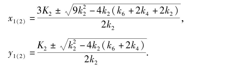
Corollary 2 ’ System (2)’has two infinite singularities. Their coordinarates are P(1,0,0),S(0,1,0), S(0,1,0) must be unstable node. As for the P(1,0,0):if 2 k 4 + k 6 > 0,the P is a (right stable) node (left) saddle point; if 2 k 4 + k 6 < 0,the P is a(right) saddle (Left stable) node.
Corollary 3 ’ Suppose k 2 < 0, k 6 + 2 k 4 < 0,,if k 2 -4( k 6 + 2 k 4 )< 0, the phase portrait of system (2)’ is Fig. 1 (1);if k 2 -4 ( k 6 -2 k 4 )= 0, the phase portrait of system(2)’ is Fig. 1(2);if k-4( k-2k) > 0,the phase portrait of system (2)’ is Fig. 1(3).
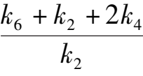
Corollary 4’ Suppose k 2 < 0, k 6 + 2 k 4 > 0, k 6 + k 2 + 2 k 4 < 0, the phase portrait of system (2)’ is Fig. 2(1).
Corollary 5 ’ Suppose k 2 < 0, k 6 + k 2 + 2 k 4 > 0, k 6 + 2 k 2 + 2 k 4 < 0, the phase portrait of system(2)’ is Fig. 3(1).
Corollary 6 ’ Suppose k 2 < 0, k 6 + 2 k 2 + 2 k 4 > 0, the phase portrait of system(2)’ is Fig. 4(1).
Corollary 7 ’If k 2 < 0, k 6 + 2 k 4 = 0, system(2)’ degenerates into the case x · = 0;if k 2 < 0, k 6 + k 2 + 2 k 4 = 0, the phase portrait of system(2)’ is Fig. 5; if k 2 < 0, k 6 +2 k 2 + 2 k 4 = 0,the phase portrait of system(2)’ is Fig. 6.
The proofs of Corollary 1’-7’ are similar to those of Corollary 1-7,so they are omitted.
Summing up the above, we obtain a theorem as the following.
Theorem
2
The sufficient and necessary condition of the existence of elliptic solution of system
 , which contacts both axes, is that the system can be expressed in the form of system (2)(0 < |
α
| < 1) or the form of system (2)’(
α
= 0). At this time, the elliptic equation is (1). Its topological classification only has eight types.They are the Fig. 1 (1),1 (2),1 (3),2 (1),3 (1),4 (1),5,6 respectively. Their parameter condition is indicated by Fig. 7(0 < |
α
| < 0) and Fig. 8(
α
= 0) separately.
, which contacts both axes, is that the system can be expressed in the form of system (2)(0 < |
α
| < 1) or the form of system (2)’(
α
= 0). At this time, the elliptic equation is (1). Its topological classification only has eight types.They are the Fig. 1 (1),1 (2),1 (3),2 (1),3 (1),4 (1),5,6 respectively. Their parameter condition is indicated by Fig. 7(0 < |
α
| < 0) and Fig. 8(
α
= 0) separately.
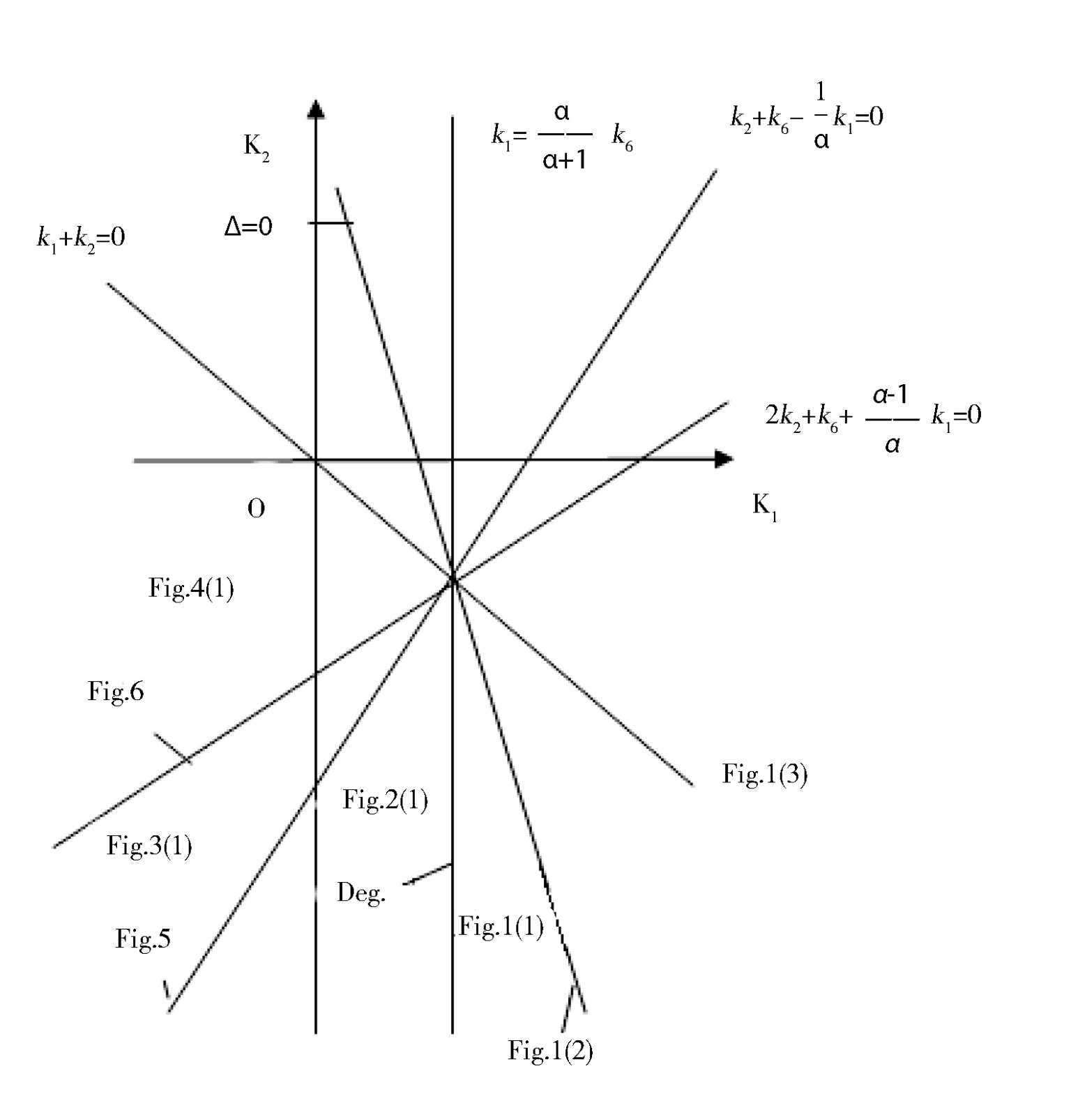
Fig. 7.
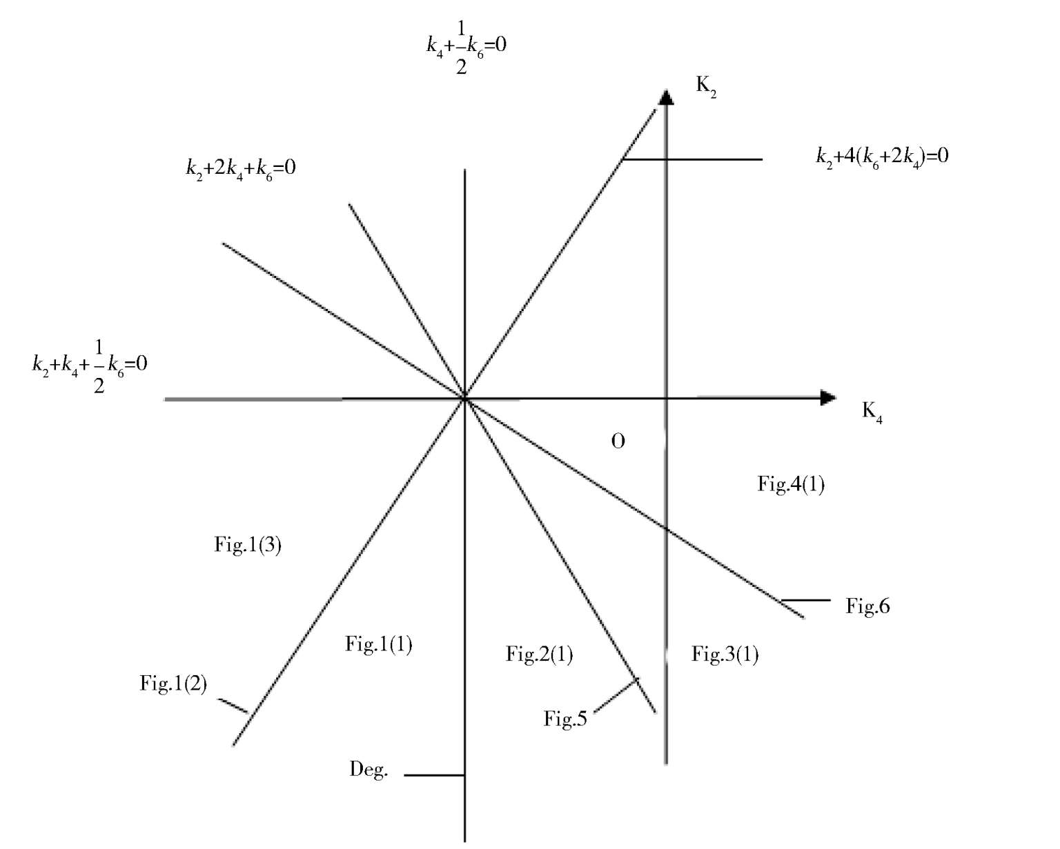
Fig. 8.
Note: If we consider system (2) or (2)’ as a mathematical model of species x and y, which restrict each other, only Fig. 4(1) has practical meaning. In this time,system (2) under the condition
k
1
+
k
2
< 0,
k
6
+ 2
k
2
+
 k
1
> 0,or system (2)’under the condition
k
2
< 0,
k
6
+ 2
k
2
+ 2
k
4
> 0,after a transformation
x
→-
x
,
y
→-
y
,these systems will be global asymptotic stable to point C in the first quadrant. See Fig.4(1).
k
1
> 0,or system (2)’under the condition
k
2
< 0,
k
6
+ 2
k
2
+ 2
k
4
> 0,after a transformation
x
→-
x
,
y
→-
y
,these systems will be global asymptotic stable to point C in the first quadrant. See Fig.4(1).
Except for the above case, all the other cases of system (2) or (2)’ have only two possibilities: one is that they are unbounded system in the first quadrant and the other is that either x or y will become extinct.
[1]Huang Qiyu, The algebraic curve cycle of a differential system with line solution Acta.Math. Appl. Sinica. , Vol. 8, No. 2,1985,173-181.
[2]Shen Boqian and Zhang Cheng, The limit cycles for the cubic kolmogorov system with a centred quadratic algebraic trajectory (to appear).
[3]Ye Yanqian etc. ,Theory of limit cycles,Shanghai Science and Technology Press,1984,248-249.
生物数学学报
1993,8(2):57-64