
下载掌阅APP,畅读海量书库
立即打开


 轨线的拓扑分类
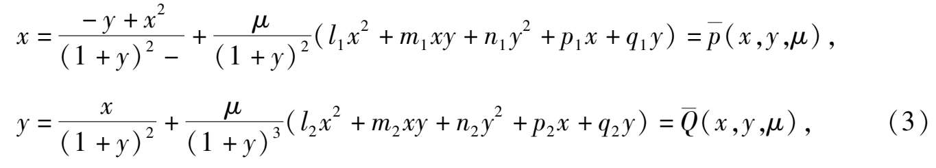
 Wtthelliptic Solution which Contact Both Axes
Abstract : In this paper we have studied the phase portrait of the kolmogorov cubic system E 3 2 with an elliptic solution which contacts both the axes. We have proved that there are altogether eight types of the topological structure of this system. Besides, if we consider this system as a mathematical model, among these eight types of topological structure of the system, only one type has practical significance.
Article [1] discussed that the kolmogorov cubic system with an elliptic solution can only possibly have periodic region, but can not have any limit cycles. Article [2]discussed that the kolmogorov cubic system with an elliptic solution which contacts both the axes can possibly have limit cycles. Article [2] only made this system with a weak focus by means of an example with a practical system and proved the existence of the limit cycles by using the Hopf bifurcation.
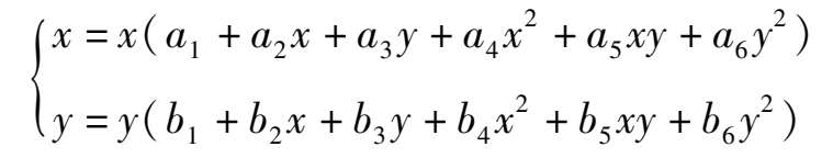
But about the topological structure of the tvajectories of this type of system, we know nothing at all. Actually for the kolmogorov cubic system which connects closely with practice, the more important thing is to study the phase portrait of this system. As it is very difficult to study the phase portrait of general kolmogorov cubic system,according to the principle from particularity to generality, we begin to discuss only the phase portrait of the particular kolmogorov cubic as in the following.
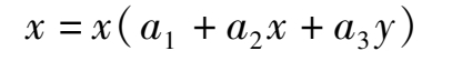

We will prove that there are altogether eight types of the topological structure of these systems. After a scale transformation, the elliptic equation contacting with two axes changes to the simpler form.

Here | α | < 1. When α = 0, the ellipse becomes a circle. It is located in the first quadrant.
Theorem
1
The sufficient and necessary condition of the existence of elliptic solution (1)(
α
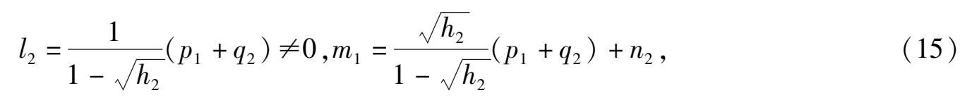
≠0) of the system
 is that the system can be expressed in the following form.
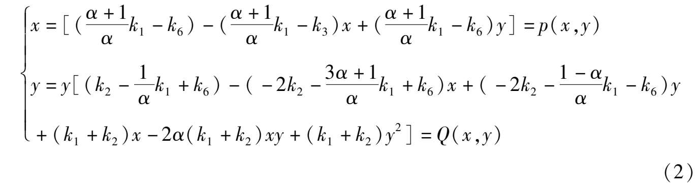
Proof Form article [2] we know that the sufficient and necessary condition of the existence of elliptic solution (1) of system.
is that the system can be expressed in the following form.
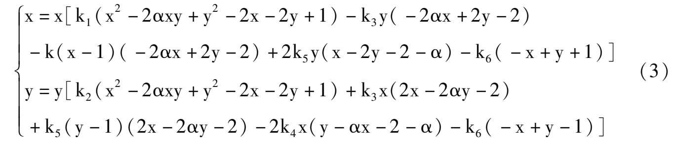
Substitute to system (3),we obtain system (2) immediately.
We can suppose k 1 + k 2 ≠0. If k 1 + k 2 = 0, then system (2) will degenerate into a quadratic system. If k 1 + k 2 > 0,by a transformation t →- t ,it can be changed to k 1 + k 2 < 0. Hence we can suppose k 1 + k 2 < 0 in system (2).
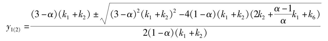
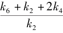
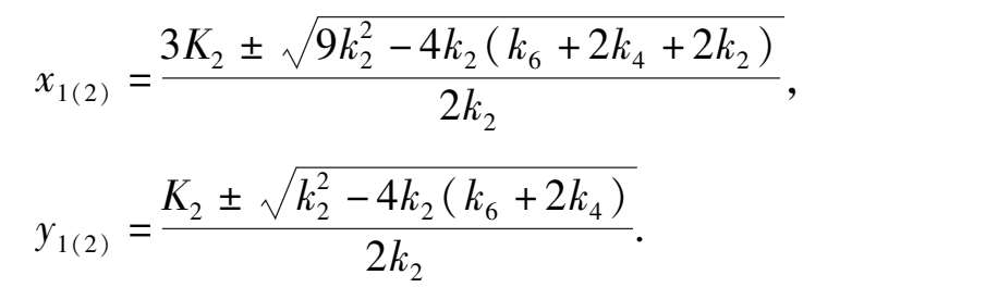
Corollary 1 System (2) has not more than six finite singularities, their coordinates are
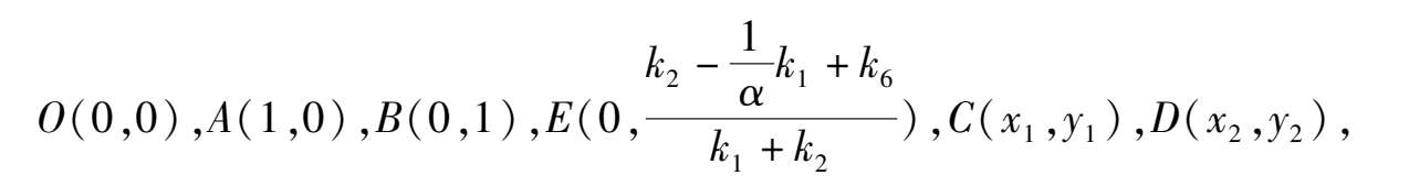
here
The proof is omitted.
Corollary
2
System (2) has two infinite singularities. Their coordinates are P(1,0,0). S(0,1,0),S(0,1,0)must be an unstable node. As for the P(1,0,0): if
 k
1
-
k
6
< 0,then the P(1,0,0) is a (right stable) node (left) saddle point; if
k
1
-
k
6
< 0,then the P(1,0,0) is a (right stable) node (left) saddle point; if
 k
1
-
k
6
> 0,then the P(1,0,0) is a (right) saddle (left stable) node.
k
1
-
k
6
> 0,then the P(1,0,0) is a (right) saddle (left stable) node.
Proof
After a transformation x =
 ,y =
,y =
 for system (2),we obtain
If use the transformation x =
 ,y =
,y =
 for system (2),we obtain
Because α 2 -1 < 0, system (2) has only two infinite singularities P (1,0,0) and S (0,1,0). Observing system (4) and (5),we can know at once that the properties of P and S as in Corollary 2 are correct.
In order to study the location and properties of finite singularities, we discuss the four different conditions separately.
(1)Point E is located at Y axis and above the B(1,0),which is
 >1 ,
>1 ,
namely
k
6
-
 k
1
< 0.
k
1
< 0.
Corollary
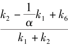
3
Suppose
k
1
+
k
2
< 0,
k
6
-
 k
1
< 0, Again
k
1
< 0, Again
1)if
Δ
= (1 +
α
)
2
(
k
1
+
k
2
)
2
-4(1-
α
)(
k
1
+
k
2
)(
k
6
-
 k
1
)> 0,namely
k
1
)> 0,namely
then the phase portrait of system (2) is indicated in Fig. 1(1);
2) if Δ < 0,namely
then the phase portrait of system (2) is Fig. 1(2);
3) if Δ < 0,namely
then the phase portrait of system (2) is Fig. 1(3).
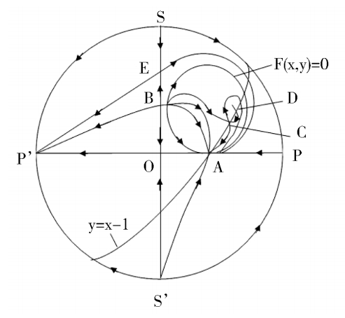
(1)
(2)
(3)
(4)
Fig. 1.
Proof
We had known that E is located at Y axis, and above B(1,0). We will consider the location about C(
x
1
,
y
1
) and D(
x
2
,
y
2
). When
k
6
-
 k
1
< 0, because 4(1-
α
)(
k
1
+
k
2
)(
k
6
-
k
1
< 0, because 4(1-
α
)(
k
1
+
k
2
)(
k
6
-
 k
1
)> 0
y
2
>
y
1
> 0, namely C and D which locate on
y
=
x
-1,they are in the first quadrant. Further we deduce that 0 <
y
1
<
y
2
<
k
1
)> 0
y
2
>
y
1
> 0, namely C and D which locate on
y
=
x
-1,they are in the first quadrant. Further we deduce that 0 <
y
1
<
y
2
<
 ,where
 is a ordinate of the intersection of the straight line
y
=
x
-1 and ellipse(1),so C and D are located inside ellipse(1) and the C is located between A and D.
is a ordinate of the intersection of the straight line
y
=
x
-1 and ellipse(1),so C and D are located inside ellipse(1) and the C is located between A and D.
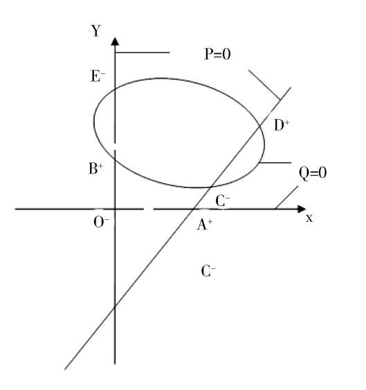
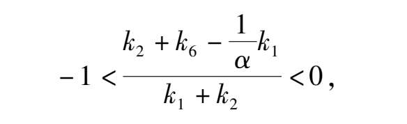
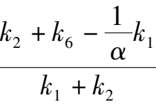
We discuss the properties of these finite singularities. Fram system(2),we know that the P(x,y) = 0 are two straight lines x = 0 and y = x -1;while the Q(x,y) = 0 is a straight line y = 0 and an ellipse. When Δ > 0, the ellipse pass through these four singularities B. C. D. E. as shown in figure1(4). According to article [3],we know that the index of O. E. C. is-1,and the index of A. B. D. is + 1. It is easy to know that they are elementary singularities, so the Fig. 1(1) is correct, except that the stability of the point D remains to be distinguished.
A s fo r t h e p o i n t D ,w e h a v e (
P
x
+
Q
y
)
D
=
 k
1
-
k
6
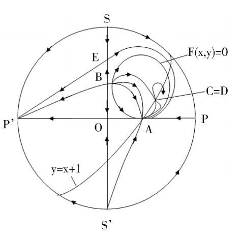
> 0, Therefore D i s a n unstable focus (node) point. When Δ = 0,the point C and D coincide and become one point. Now, for the system (2) we obtain the matrix.
k
1
-
k
6
> 0, Therefore D i s a n unstable focus (node) point. When Δ = 0,the point C and D coincide and become one point. Now, for the system (2) we obtain the matrix.
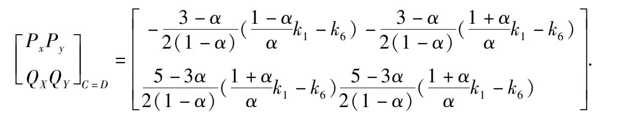
Because these two column elements are in proportion, and(
P
x
+
Q
y
)
C
= D=
 k
1
-
k
6
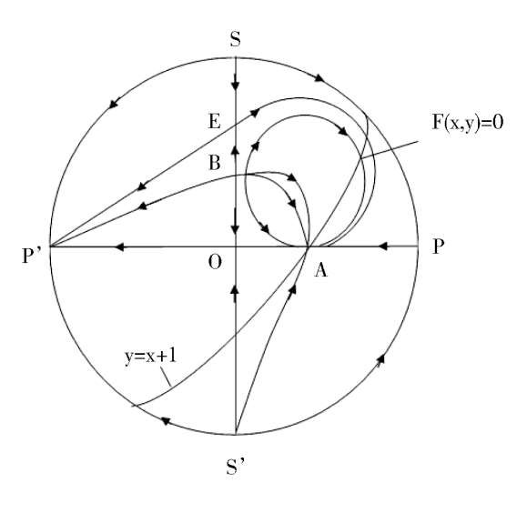
> 0, therefore C and Dcoincide and become a saddle(unstable) node, as shown in figue1(2). When Δ < 0,C and D disappeared. Its phase portrait must be indicated by figue1 (3).
k
1
-
k
6
> 0, therefore C and Dcoincide and become a saddle(unstable) node, as shown in figue1(2). When Δ < 0,C and D disappeared. Its phase portrait must be indicated by figue1 (3).
Note the proof of Corollary 3. If we distinguish the property of every finite singularity. Through calculation, the result will be the same. But if we do so, there will be a large amount of calculation and a great length of space.
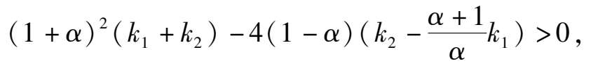
(2) Point E is located at Y axis and between B and O, that is 0 <
 < 1, namely
k
2
+
k
2
-
< 1, namely
k
2
+
k
2
-
 k
< 0,and
k
6
-
k
< 0,and
k
6
-
 k
1
> 0.
k
1
> 0.
Corollary
4
Suppose
k
1
+
k
2
< ,
k
6
-
 k
1
> 0,
k
2
+
k
6
-
k
1
> 0,
k
2
+
k
6
-
 k
1
< 0 ,the phaseportrait of system (2) is indicated in Fig. 2 (1).
k
1
< 0 ,the phaseportrait of system (2) is indicated in Fig. 2 (1).
Proof
We had known that the E is located at y axis between B and O. As for the locating of C(
x
1
,
y
1
),D(
x
2
,
y
2
),because
k
6
+ 2
k
2
-
 k
1
=
k
6
+
k
2
-
k
1
=
k
6
+
k
2
-
 k
1
+ (
k
1
+
k
2
) < 0,we can deduce that 0 <
x
1
<
x
2
,
y
1
< 0
k
1
+ (
k
1
+
k
2
) < 0,we can deduce that 0 <
x
1
<
x
2
,
y
1
< 0
 <
y
2
easily, namely C is located in the fourth quadrant and D is located above the ellipse(1).As shown in Fig.2(2).
<
y
2
easily, namely C is located in the fourth quadrant and D is located above the ellipse(1).As shown in Fig.2(2).
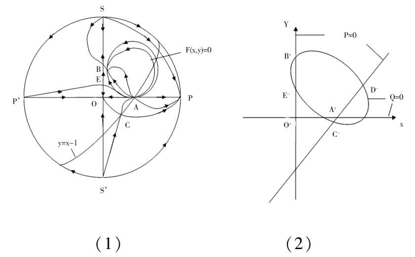
Fig. 2.
According to article [3],we know that Fig. 2(1) is exactly correct.
(3)Point E is located at negative y axis and above the straight line y = x-1, that is
namely
Corollary
5
Suppose
k
1
+
k
2
< 0,
k
6
+
k
2
-
 k
1
> 0,
k
6
+ 2
k
2
-
k
1
> 0,
k
6
+ 2
k
2
-
 k
1
< 0,thephase portrait of system (2) is indicated in Fig. 3 (1).
k
1
< 0,thephase portrait of system (2) is indicated in Fig. 3 (1).
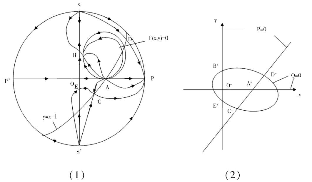
Fig. 3.
Proof We had known that E is located any axis and between 0 and straight line y= x-1. As for the location of C ( x 1 , y 1 ),D( x 2 , y 2 ), because

we can deduce that
x
1
> 0,
x
2
> 0,
y
1
< 0 <
 <
y
2
easily, so C is located in the fourth quadrant and the D is located above the ellipse (1),as shown in Fig. 3 (2).According to article [3],we know that Fig. 3(1) is exactly correct.
<
y
2
easily, so C is located in the fourth quadrant and the D is located above the ellipse (1),as shown in Fig. 3 (2).According to article [3],we know that Fig. 3(1) is exactly correct.
(4)Point E is located at negative y axis and below the straight line y = x-1,that is
 <-1, namely
k
6
+ 2
k
2
-
<-1, namely
k
6
+ 2
k
2
-
 k
1
> 0.
k
1
> 0.
Corollary
6
Suppose
k
1
+
k
2
< 0,
k
6
+ 2
k
2
-
 k
1
> 0, the phase portrait of system (2) is indelicate in Fig. 4(1).
k
1
> 0, the phase portrait of system (2) is indelicate in Fig. 4(1).
Proof We had known that E is located at negative y axis and below the straight line y = x-1.
As for the location of C( x 1 , y 1 ),D( x 2 , y 2 ), because
we can deduce that
so the C is located in the third quadrant and the D is located above the ellipse(1),as shown in Fig. 4 (2). According to article [3],we know that Fig. 4 (1 ) is exactly correct only the stability of C remains to be distinguished.
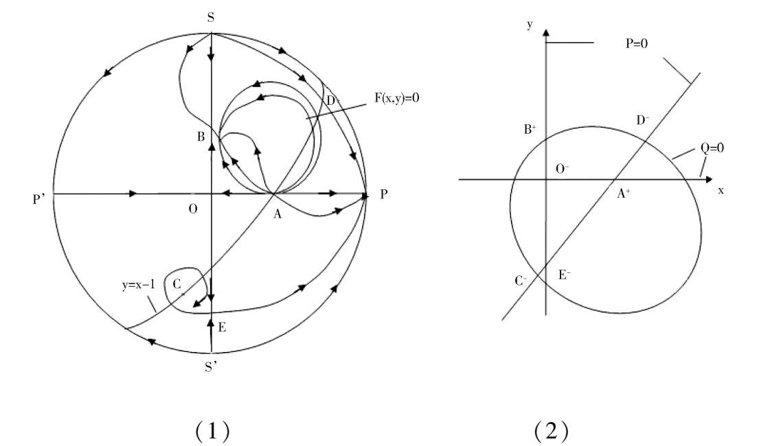
Fig. 4.
Since(
P
x
+
Q
y
) C =
 k
1
-
k
6
< 0, C is stable focus ( node).( If there have limit cycles surrounding the point C, the number of limit cycles must be even. But we estimate that it will not happen. ).
k
1
-
k
6
< 0, C is stable focus ( node).( If there have limit cycles surrounding the point C, the number of limit cycles must be even. But we estimate that it will not happen. ).
We go on with our work to study the following three cases:i)E coincides to B ( namely the condition
k
6
-
 k
1
= 0),ii) E coincides to D (namely the condition
k
6
+
k
2
-
k
1
= 0),ii) E coincides to D (namely the condition
k
6
+
k
2
-
 k
1
= 0),iii) E is located on straight y = x-1,for this moment E coincides to C(namely the condition
k
6
+ 2
k
2
+
k
1
= 0),iii) E is located on straight y = x-1,for this moment E coincides to C(namely the condition
k
6
+ 2
k
2
+
 k
1
= 0).
k
1
= 0).
Corollary
7
If
k
1
+
k
2
< 0,
k
6
-
 k
1
= 0, the system (2) degenerates into the case
k
1
= 0, the system (2) degenerates into the case
 = 0;I f
k
1
+
k
2
<0 ,
k
6
+
k
2
-
= 0;I f
k
1
+
k
2
<0 ,
k
6
+
k
2
-
 k
1
= 0, the phase portrait of system (2) is indicated by Fig. 5;If
k
1
+
k
2
< 0,
k
6
+
k
2
+
k
1
= 0, the phase portrait of system (2) is indicated by Fig. 5;If
k
1
+
k
2
< 0,
k
6
+
k
2
+
 k
1
= 0, the phase portrait of system(2) is indicated by Fig. 6.
k
1
= 0, the phase portrait of system(2) is indicated by Fig. 6.
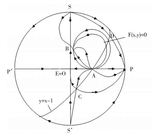
Fig. 5.
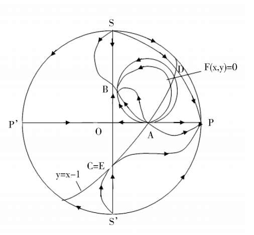
Fig. 6.
Finally, we will have to discuss continuously. When α = 0, then equation (1) change to a circle

The corresponding system (2) will change to the system
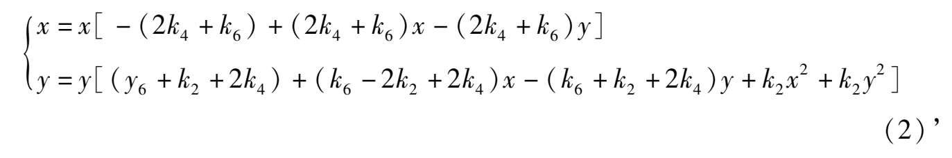
Without loss of generality, we can let k 2 < 0.(If = 0,system(2)’ can degenerate to a quadric system).
Corresponding to system (2),we have some corollaries of system(2)’ as in the following.
Corollary
1
’ System (2 )’ has not more than six finite singularities. Their coordinates are O(0,0),A(1,0),B(0,1),E(0,
 ), C(
x
1
,
y
1
),D(
x
2
,
y
2
), here
), C(
x
1
,
y
1
),D(
x
2
,
y
2
), here
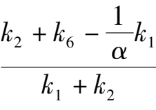
Corollary 2 ’ System (2)’has two infinite singularities. Their coordinarates are P(1,0,0),S(0,1,0), S(0,1,0) must be unstable node. As for the P(1,0,0):if 2 k 4 + k 6 > 0,the P is a (right stable) node (left) saddle point; if 2 k 4 + k 6 < 0,the P is a(right) saddle (Left stable) node.
Corollary 3 ’ Suppose k 2 < 0, k 6 + 2 k 4 < 0,,if k 2 -4( k 6 + 2 k 4 )< 0, the phase portrait of system (2)’ is Fig. 1 (1);if k 2 -4 ( k 6 -2 k 4 )= 0, the phase portrait of system(2)’ is Fig. 1(2);if k-4( k-2k) > 0,the phase portrait of system (2)’ is Fig. 1(3).
Corollary 4’ Suppose k 2 < 0, k 6 + 2 k 4 > 0, k 6 + k 2 + 2 k 4 < 0, the phase portrait of system (2)’ is Fig. 2(1).
Corollary 5 ’ Suppose k 2 < 0, k 6 + k 2 + 2 k 4 > 0, k 6 + 2 k 2 + 2 k 4 < 0, the phase portrait of system(2)’ is Fig. 3(1).
Corollary 6 ’ Suppose k 2 < 0, k 6 + 2 k 2 + 2 k 4 > 0, the phase portrait of system(2)’ is Fig. 4(1).
Corollary 7 ’If k 2 < 0, k 6 + 2 k 4 = 0, system(2)’ degenerates into the case x · = 0;if k 2 < 0, k 6 + k 2 + 2 k 4 = 0, the phase portrait of system(2)’ is Fig. 5; if k 2 < 0, k 6 +2 k 2 + 2 k 4 = 0,the phase portrait of system(2)’ is Fig. 6.
The proofs of Corollary 1’-7’ are similar to those of Corollary 1-7,so they are omitted.
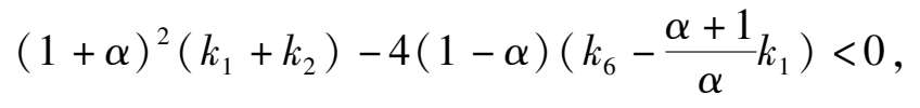
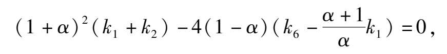
Summing up the above, we obtain a theorem as the following.
Theorem
2
The sufficient and necessary condition of the existence of elliptic solution of system
 , which contacts both axes, is that the system can be expressed in the form of system (2)(0 < |
α
| < 1) or the form of system (2)’(
α
= 0). At this time, the elliptic equation is (1). Its topological classification only has eight types.They are the Fig. 1 (1),1 (2),1 (3),2 (1),3 (1),4 (1),5,6 respectively. Their parameter condition is indicated by Fig. 7(0 < |
α
| < 0) and Fig. 8(
α
= 0) separately.
, which contacts both axes, is that the system can be expressed in the form of system (2)(0 < |
α
| < 1) or the form of system (2)’(
α
= 0). At this time, the elliptic equation is (1). Its topological classification only has eight types.They are the Fig. 1 (1),1 (2),1 (3),2 (1),3 (1),4 (1),5,6 respectively. Their parameter condition is indicated by Fig. 7(0 < |
α
| < 0) and Fig. 8(
α
= 0) separately.
Fig. 7.
Fig. 8.
Note: If we consider system (2) or (2)’ as a mathematical model of species x and y, which restrict each other, only Fig. 4(1) has practical meaning. In this time,system (2) under the condition
k
1
+
k
2
< 0,
k
6
+ 2
k
2
+
 k
1
> 0,or system (2)’under the condition
k
2
< 0,
k
6
+ 2
k
2
+ 2
k
4
> 0,after a transformation
x
→-
x
,
y
→-
y
,these systems will be global asymptotic stable to point C in the first quadrant. See Fig.4(1).
k
1
> 0,or system (2)’under the condition
k
2
< 0,
k
6
+ 2
k
2
+ 2
k
4
> 0,after a transformation
x
→-
x
,
y
→-
y
,these systems will be global asymptotic stable to point C in the first quadrant. See Fig.4(1).
Except for the above case, all the other cases of system (2) or (2)’ have only two possibilities: one is that they are unbounded system in the first quadrant and the other is that either x or y will become extinct.
[1]Huang Qiyu, The algebraic curve cycle of a differential system with line solution Acta.Math. Appl. Sinica. , Vol. 8, No. 2,1985,173-181.
[2]Shen Boqian and Zhang Cheng, The limit cycles for the cubic kolmogorov system with a centred quadratic algebraic trajectory (to appear).
[3]Ye Yanqian etc. ,Theory of limit cycles,Shanghai Science and Technology Press,1984,248-249.
生物数学学报
1993,8(2):57-64
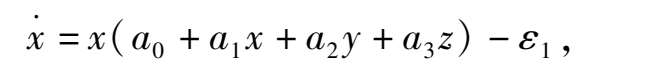
摘 要 : 本文对具有某些代数曲面解的具有常收获率和常投放率的三种群 Volterra 模型在 R 3 + 内的相图进行了分析 , 并举出了一些具体例子 .
关键词 : 三种群 Volterra 模型 , 收获率 , 投放率 , 相图
三维系统的相图要比二维系统的相图复杂得多,对于二维系统相图的分析虽然也不是太容易,但其已有的成果可以说已不胜枚举.而对于三维系统的相图分析却很少见.
其主要原因是难度太大,对于一些实际问题的具体三维系统模型,在
 (第一卦限)内极限环的存在性、唯一性,或平衡点的稳定性全局稳定性等,虽然也有过不少结果.例如极限环存在性方面的结果如文〔1,2〕等,平衡点稳定性,或全局稳定的如文〔3,4〕等,但是在
 轨线的分布与走向状况却知之甚少,而
 内轨线分布和走向恰恰是解决实际问题时所最需要的.比如对给的初始点,那些变元最终走向灭绝,那些变元始终保持存在,且将稳定在什么位置上,这些都正是实际所最需要加以解决的问题.
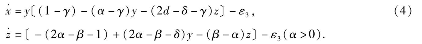
文〔5〕曾证明过系统:
 =
x
(1-
x
-
αy
-
βNz
) +
ε
,
=
x
(1-
x
-
αy
-
βNz
) +
ε
,
 =
y
(1 +
βx
-
y
-
az
) +
ε
,
=
y
(1 +
βx
-
y
-
az
) +
ε
,
 =
z
(1-
αx
-
βy
-
z
) +
ε
=
z
(1-
αx
-
βy
-
z
) +
ε
在满足一定条件时存在极限环,但极限环的可能形状,区域 R 3 +内轨线的可能分布和走向方面仍一无所知.本文将考虑以下系统
并试图探索此类系统在
 内轨线可能的分布和走向.当然对一般情况下的系统(1),要较全面地解决此问题难度很大,简直无法下手.所以现在我们只研究当系统(1)具有某些代数曲面解时的特殊情形.因为这时我们就有可能将此三维系统转化为二维系统来进行研究.尽管对这类特殊的系统(1)轨线的研究结果不能代表一般的系统(1),但至少可以知道系统(1)的轨线可以出现何种类型的拓扑结构.也可以为进一步对一般的系统(1)的研究提供线索和信息.
我们有以下定理:
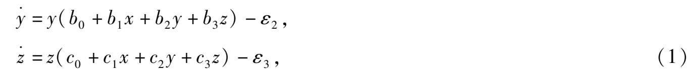
定理 1 系统(1)具有平面解 F ( x , y , z ) = x + y + z -1 = 0 的充要条件是此系统可表示成以下形式:
这里 A , B , C , b 1 , a 3 , c 2 均为任意常数, D = ε 1 + ε 2 + ε 3 .
证 设系统(1)具有平面解 F ( x , y , z ) = x + y + z -1 = 0,则对系统(1)有
即

比较系数得:
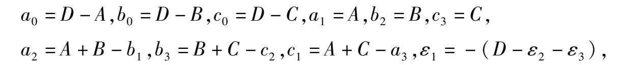
代入系统(1)即得系统(2).条件的充分性证毕.条件的必要性是显然的.证毕.
我们假设系统(2)的三种群都具有正出生率,不妨都设为 1,即设 D - A = 1, D - B = 1, D - C = 1,则系统(2)变成以下形式:
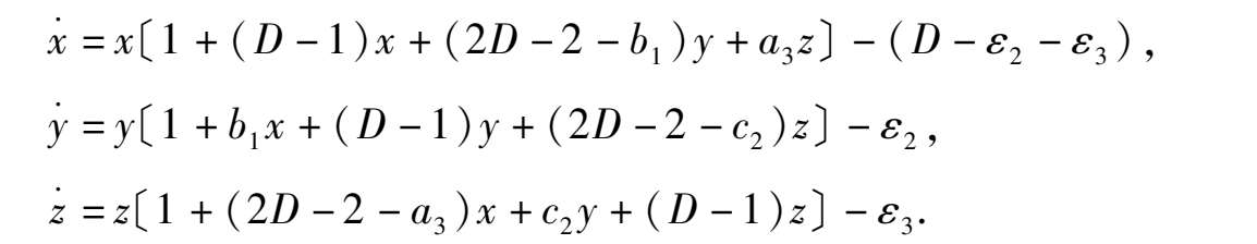
因三种群的密谋制约项必为负,所以可设 D -1 =- α ( α > 0).并记 b 1 =- γ , c 2 =- δ , α 3 =- β ,于是此系统又可写成:
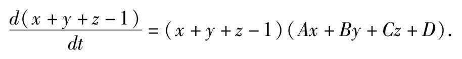
因为

系统(3)有初积分为:

其中 C 是任意常数.
引理
1 系统(3)在第一卦限
 是有界系统.
证
因
 (
x
+
y
+
z
-
N
) =-(
x
+
y
+
z
-1)〔
α
(
x
+
y
+
z
-1)+ (2
α
-1)〕,
(
x
+
y
+
z
-
N
) =-(
x
+
y
+
z
-1)〔
α
(
x
+
y
+
z
-1)+ (2
α
-1)〕,
所以

当
N
充分大时
 (
x
+
y
+
z
-
N
)
x
+
y
+
z
=
N
< 0,证毕.
(
x
+
y
+
z
-
N
)
x
+
y
+
z
=
N
< 0,证毕.
引理 2 系统(3)
当0 <
α
<
 时,
时,
 (
x
+
y
+
z
) =-
(
x
+
y
+
z
) =-
 ,
,
 (
x
+
y
+
z
) = 1,
(
x
+
y
+
z
) = 1,
当
 ≤
α
< 1 时,
≤
α
< 1 时,
 (
x
+
y
+
z
) = 1,
(
x
+
y
+
z
) = 1,
 (
x
+
y
+
z
) =-
(
x
+
y
+
z
) =-
 ,
,
当
α
> 1 时,
 (
x
+
y
+
z
) = 1.
(
x
+
y
+
z
) = 1.
证明略.
引理 2 说明系统(3)有两个平行面解,即平面解Ⅰ:
x
+
y
+
z
= 1,和平面解Ⅱ:
x
+
y
+
z
+
 = 0,当0 <
α
<
= 0,当0 <
α
<
 时,Ⅰ是负向不变集;Ⅱ是正向不变集,当
 <
α
<1时,则反之.当
α
> 1时Ⅰ是正向不变集.当
α
=
<
α
<1时,则反之.当
α
> 1时Ⅰ是正向不变集.当
α
=
 时,Ⅰ与Ⅱ重合,这时面向原点的一侧属负向不变集,背向原点的一侧属正向不变集.
对系统(3)设 x = 1- y - x 得
这是关于
y
,
z
均具有常收获或常投放的Volterra系统.如对系统(3)作变换
x
=-
 -
y
-
z
得
-
y
-
z
得
这也是关于 y , z 均具常收获或常投放的Volterra系统.
如果我们能得出系统(4)和(5)在平面(
y
,
z
)上第一象限内的相图,那么根据引理 2,我们就不难得知系统(3)在
 内轨线分布和走向状况.二维系统(4)和(5)是可以存在极限环的,从而可知三维系统(3)也是可以存在极限环的.但是仅靠定性的方法要对一般的系统(4)和(5)给出它们丰在极限环的精确条件,难度是极大的,如果要进一步研究系统(4)和(5)的在第一象限内各种可能的轨线的拓朴结构,难度更大.由于我们现在不想纠缠在对一般二维系统(4)与(5)的冗长的讨论上,所以本文只想举一些具体的数字系统的例子来说明三维系统(3)在
 内可能出现的轨线分布和走向.这对进一步揭示系统(3)的轨线结构是有益的.
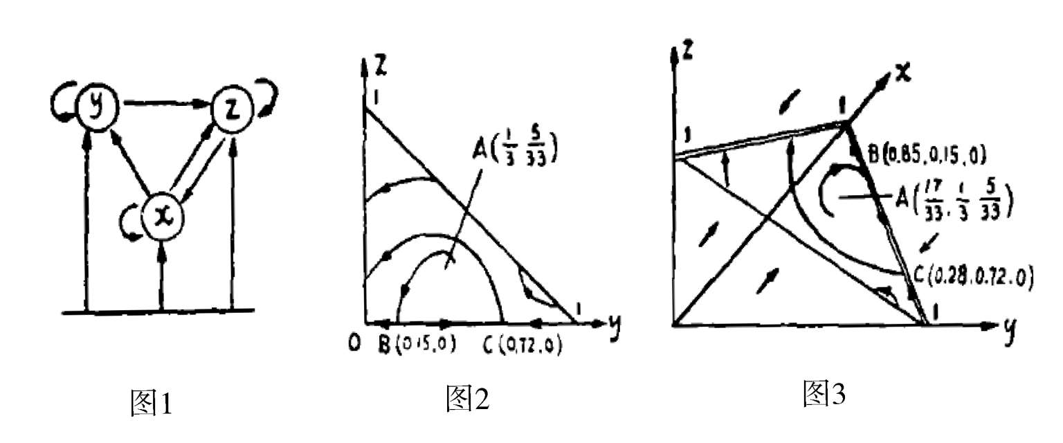
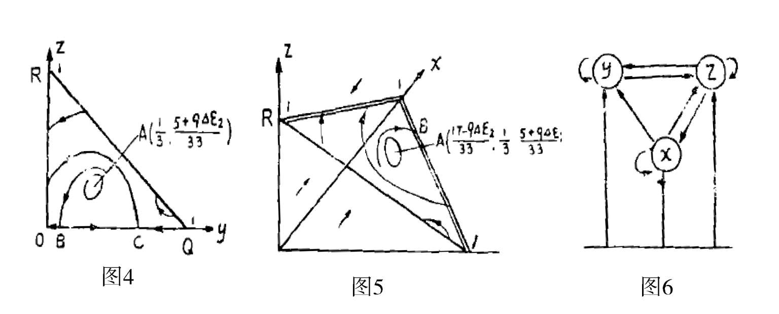
例
1令
α
= 2,
β
= 2,
δ
=-1,
γ
=-6,
ε
1
=
 ε
3
= 0,
这时系统(3)形为
ε
3
= 0,
这时系统(3)形为
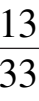
系统(6)中的种群 x , y , z 之间的关系如图 1 所示,其中对 x 有常投放,对 y 有常收获.系统(6)通过变换 x = 1- y - z 得二维系统(4)形如
系统(7)在第一象限有唯一奇点
A
(
 ,
,
 ),它位于区域
D
:{(
y
,
z
) |
y
> 0,
z
>0,
y
+
z
< 1}内.且易验知
A
为系统(7)的一阶不稳定细焦点.系统(7)在第一象限内的相图如图2 所示.因
α
> 1,从引理2 知系统(6)在
),它位于区域
D
:{(
y
,
z
) |
y
> 0,
z
>0,
y
+
z
< 1}内.且易验知
A
为系统(7)的一阶不稳定细焦点.系统(7)在第一象限内的相图如图2 所示.因
α
> 1,从引理2 知系统(6)在
 的轨线当
t
→∞时均趋向于平面解
x
+
y
+
z
-1 = 0,所以系统(6)在
的轨线当
t
→∞时均趋向于平面解
x
+
y
+
z
-1 = 0,所以系统(6)在
 内轨线的分布和走向大致如图 3所示.
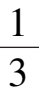
如在系统(6)的基础上令
ε
2
减小,即令
α
= 2,
β
= 2,
δ
=-1,
γ
=-6,
ε
2
=
 -
Δε
2
(0 <
Δε
2
< 1)则系统(6)和系统(7)分别变成
-
Δε
2
(0 <
Δε
2
< 1)则系统(6)和系统(7)分别变成
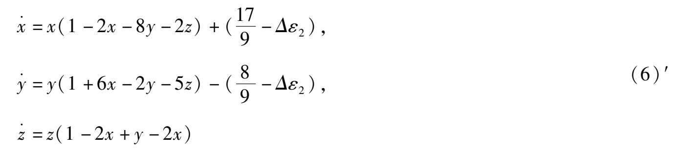
和
由于这时系统(7)′在第一象限的唯一奇点
A
(
 ,
,
 )变成稳定粗焦点,所以
A
外围出现了一个不稳定极限环.其相图变成图 4 所示.从而系统(6)′在
)变成稳定粗焦点,所以
A
外围出现了一个不稳定极限环.其相图变成图 4 所示.从而系统(6)′在
 也出现了唯一不稳定极限环,它位于平面解
x
+
y
+
z
-1 = 0 上.如图 5 所示.
也出现了唯一不稳定极限环,它位于平面解
x
+
y
+
z
-1 = 0 上.如图 5 所示.
注
1 在系统(7)′和(6)′中,当 0 <
Δε
2
< 1 时极限环存在(唯一),不必一定限制
Δε
2
为充分小,实际上当
Δε
2
增大到
 时,系统(7)′在第一象限将全局稳定于点
A
(
时,系统(7)′在第一象限将全局稳定于点
A
(
 ,
,
 ).所以在间向0<
Δε
2
<
).所以在间向0<
Δε
2
<
 必存在使得系统(7)′在
A
外围存在弓形分界线环的值.由于系统(7)′对
Δε
2
不构成旋转向量场,所以这个值不是唯一的.如设其中最小的值为
Δε
2
,则当 0 <
Δε
2
<
Δε
2
时,系统(7)′必存在(唯一)不稳定极限环,从而系统(6)′也存在(唯一)不稳定极限环.
必存在使得系统(7)′在
A
外围存在弓形分界线环的值.由于系统(7)′对
Δε
2
不构成旋转向量场,所以这个值不是唯一的.如设其中最小的值为
Δε
2
,则当 0 <
Δε
2
<
Δε
2
时,系统(7)′必存在(唯一)不稳定极限环,从而系统(6)′也存在(唯一)不稳定极限环.
注 2 系统(6)′当 0 < Δε 2 < Δε 2 时的不稳定极限环位于平面 x + y + z -1 = 0 上完全有可能与图 5 中的线段 RQ 相交,也即沿某一轨线,当 t 到达某一有限时刻,种群 x 就灭绝了,但后又复生了,这不足为奇,因为 x 具有常投放率.
注
3 系统(6)′当
Δε
2
减小时,种群
x
,
y
,
z
不能共存,当
t
到达某有限时刻,
y
必灭绝,只剩下
x
和
z
,而当
Δε
2
增大时,
 内将出现稳定区域,即出现
x
,
y
,
z
共存的区域.当
Δε
2
增大到
内将出现稳定区域,即出现
x
,
y
,
z
共存的区域.当
Δε
2
增大到
 时,
时,
 内全局稳定于点
 .
.
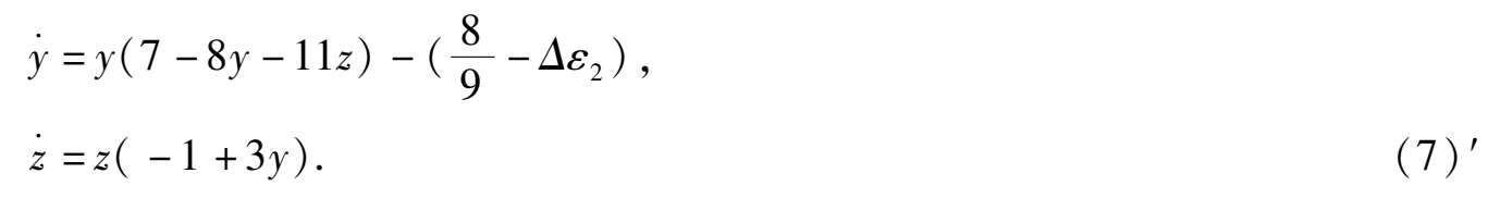
例
2令
α
=
 ,
δ
=
,
δ
=
 ,
β
=
,
β
=
 ,
γ
=-8,
ε
2
=
,
γ
=-8,
ε
2
=
 ,
ε
2
= 0,这时系统(3)形为
,
ε
2
= 0,这时系统(3)形为
系统(8)中的种群 x , y , z 之间的关系如图 6 所示,对 x 有常设放,对 y 有常收获.系统(8)通过变换 x = 1- y - z 所得系统(4)形为
系统(9)在第一象限有唯一奇点
A
(
 ,
,
 ),它位于区域
D
:{(
y
,
z
) |
y
> 0,
z
>0
y
+
z
< 1}内,
y
轴上有奇点
B
(
),它位于区域
D
:{(
y
,
z
) |
y
> 0,
z
>0
y
+
z
< 1}内,
y
轴上有奇点
B
(
 ,0)=
B
(0.916,0)和
C
(
,0)=
B
(0.916,0)和
C
(
 ,0)=
C
(0,112,0)
A
为鞍点,
B
为稳定结点,
C
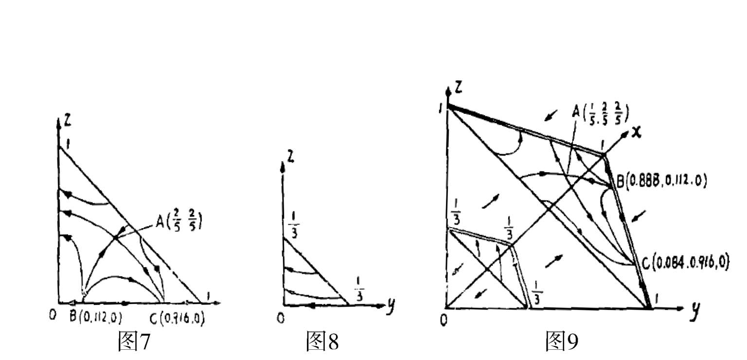
为不稳定结点.系统(9)在第一象限的相图如图 7 所示.
,0)=
C
(0,112,0)
A
为鞍点,
B
为稳定结点,
C
为不稳定结点.系统(9)在第一象限的相图如图 7 所示.
系统(8)通过变换
x
=
 -
y
-
z
所得系统(5)形为
-
y
-
z
所得系统(5)形为

系统(10)全平面只有唯一奇点
A
(
 ,-
,-
 ),在第一象限相图如图 8 所示.
因
a
=
 < 1,所以由引理 1 可知系统(8)的平面
x
+
y
+
z
-1 = 0 是正向不变集,平面
x
+
y
+
z
-
< 1,所以由引理 1 可知系统(8)的平面
x
+
y
+
z
-1 = 0 是正向不变集,平面
x
+
y
+
z
-
 = 0是负向不变集.所以系统(8)在
 的相图如图 9 所示.在
 内,平面I:
x
+
y
+
z
= 1 上侧轨线均走向平面I;在平面I和Ⅱ:
x
+
y
+
z
=
内,平面I:
x
+
y
+
z
= 1 上侧轨线均走向平面I;在平面I和Ⅱ:
x
+
y
+
z
=
 之间,轨线均远离Ⅱ而走向Ⅰ;在平面Ⅱ下侧轨线均远离Ⅱ.
注 4 系统(8)中种群 x , y , z 不能共存,根据初始点( x 0 , y 0 , z 0 )所在的位置,有以下几种不同的结果:
1)如初始点(
x
0
,
y
0
,
z
0
)位于平面Ⅱ的上侧时有两种可能性:一种是当
t
→ + ∞时,
z
灭绝,而
x
和
y
的数量稳定在(0.084,0.916);另一种是当
t
到达有限时刻
y
将灭绝而
x
,
z
仍存在着.例如当0 <
δ
≪1时初始点取在(
 +
δ
)时,
y
必当
t
于有限时刻就灭绝,
x
,
z
存在;初始点取在(
+
δ
)时,
y
必当
t
于有限时刻就灭绝,
x
,
z
存在;初始点取在(
 -
δ
)时,当
t
→∞时,
z
灭绝,而
x
,
y
稳定在(0.084,0.916),初始点位置差以毫厘,后果却不大一样.
-
δ
)时,当
t
→∞时,
z
灭绝,而
x
,
y
稳定在(0.084,0.916),初始点位置差以毫厘,后果却不大一样.
2)如初始点( x 0 , y 0 , z 0 )位于平面Ⅰ的下侧.则当 t 到达有限时刻时 y 必灭绝,而 x , z 继续存在.
以上我们只举了两个例子,如果对于系统(3)任意给定
α
,
β
,
γ
,
δ
,
ε
2
,
ε
3
的一组数,我们都可以描绘出所对应的系统(3)在
 内的轨线分布图.至于对系统(3)的一般性讨论,有待进一步研究.
参考文献
[1]Lo Sheag Dai,Noncoustant periodic solution in predatorprey systems with continuous time delay,Math,Biosci,53,1981,109-157.
[2]Gopalsamy,K. Aggarwala B. D. ,Limit cycles in two species competition with time delays,J. Aust Math Soc. Ser. B. 1980,21,148-160.
[3]Bowads J. M. and Cushing J. M. ,On the behavior of sofutions of predator- prey equations with bereditary term,Math,Biosci,1975,29,41-54.
[4]陈兰荪,数学生态模型与研究方法,科学出版社,北京,1988,310-321,205-232.
[5] Grusman W,Periodic solutions of autonomous differential equations in higher dimeasion spaces Rocky Mountain J. Math. 1977,7(3):457-466.
[6]陈兰荪,数学生态模型与研究方法,科学出版社,北京,1988,310-321,205-232.
Abstract :This paper presents the analysis of the phase portrait of three species Volterra model with the rates of constant harvest and constant invest braic curved surface solution in R 3 +It also offers some practical examples.
Keywords :Three species Volterra model,Harvest rate,Invest rate,Phase portrait.
应用数学学报
1994,17(4):592-596
本文将证明从二次系统的内含焦点的只有一个无限远高次奇点的无限大分界线环可以分支出两个极限环,或分支出一个二重极限环.
文[1]曾研究过以下二次系统的Poincare分支.

易知系统(1) μ = 0 有通积分

当 0 < h < 1 时,(2)是绕 0(0,0)的一族闭曲线;当h→ + 0 时,(2)成为一条抛物线2 y + 1- x 2 = 0;当h→-0 时,(2)成为一个孤立点 0(0,0).
系统(1) μ = 0 不是Hamilton系统,但是如果在系统(1) μ 的右边同乘以 1 /(1+ y) 3 ,变成了以下形式:
则系统(3) μ = 0 就变成了Hamilton系统. Hamilton函数为(2).现在我们可以根据文[2]考虑以下函数:
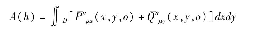
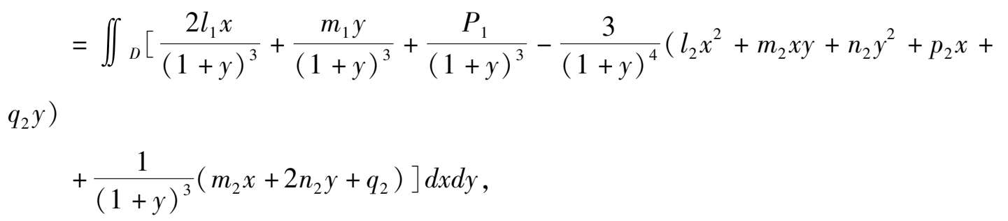
其中D表示闭曲线(2)(0 < h < 1)所围的区域,计算A( h )得
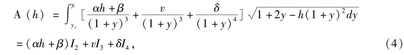
其中

这里
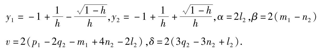
引理 1

证 先计算(5)式中的 I n .设 1 + y = z ,则

其中

则
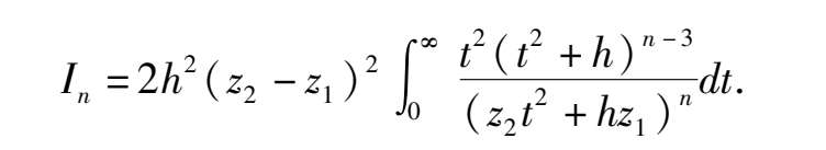
分别计算 I 2 , I 3 , I 4 得
所以
证毕.
如设21 ( γ + δ )= γ′ (6)式又可改写成以下形式

根据文献[2],我们讨论函数A( h )在区间 0 < h < 1 内零点的个数,也即讨论函数 ϕ ( h )在区间 0 < h < 1 内零点的个数.
任取 h 1 , h 2 ,0 < h 1 < h 2 < 1,使 ϕ ( h 1 )= 0, ϕ ( h 2 )= 0,即

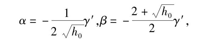
因方程组(8)中关于未知数 α , β 的系数行列式 Δ = h 1 - h 2 < 0 所以在方程组(8)中,可以解出 α , β :

定理 1 对任意给定的 h 1 , h 2 :0 < h 1 < h 2 < 1,如果系统的系统(1) μ 满足以下条件:
则当 0 < | μ |≪1 时,在原点外围存在两个极限环,它们分别位于两条闭曲线:

的充分小邻域内.
证 根据前段讨论可知,系统(1) μ 当条件(9)成立时, A ( h )在 0 < h < 1 内有两个零点 h = h 1 和 h = h 2 .而条件(10)是条件(9)的等阶条件.又
所以根据Poincar e ′分支理论 [2] ,可知本定理 1 的结论成立,证毕.
定理 2 系统(1) μ 的Poincar e ′分支至多只能分支出两个极限环.
证 任意给定 h 1 , h 2 , h 3 :0 < h 1 < h 2 < h 3 < 1,令 φ ( h i ) = 0, i = 1,2,3,也即

此方程组(12)关于未知数 α , β , γ′ 的系数行列式

所以方程组(12)只可能有零解 α = 0, β = 0, γ′ = 0,也就是说函数 ϕ ( h )也即函数 A ( h )在 0 < h < 1 内不可能存在三个零点,否则 A ( h ) = 0.证毕.
其实如果把函数
ϕ
(
h
)看作关于
 的二次多项式,则
ϕ
(
h
)在 0 <
h
< 1 上至多只有两个零点是显然的,也即定理 2 的结论是显然成立的.
的二次多项式,则
ϕ
(
h
)在 0 <
h
< 1 上至多只有两个零点是显然的,也即定理 2 的结论是显然成立的.
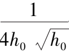
如果在定理 1 的基础上令 h 1 = h 2 = h 0 (0 < h 1 < 1)系统(1) μ 将有二重极限环出现,有以下定理.
定理 3 对任意给定的 h 0 :0 < h 0 < 1,系统的(1) μ 系数如满足以下条件:

则当 0 < | μ |≪1 时,原点外围存在二重极限环,它位于闭曲线(2y + 1- x 2 )/(1 + y) 2 = h 2 的充分小邻域内.
证 令 ϕ ( h 0 )= 0 .ϕ′ ( h 0 )= 0,也即

显然从方程组(14)中可解出
它与条件(13)等价.注意到
ϕ″
(
h
0
)=-
 γ′
≠0,所以当条件(13)成立时,
A
(
h
)在 0 <
h
< 1 内有一个二重根
h
=
h
0
.根据
γ′
≠0,所以当条件(13)成立时,
A
(
h
)在 0 <
h
< 1 内有一个二重根
h
=
h
0
.根据
 分支理论[2]可知本定理 3的结论成立.证毕.
本文以上所得的结果与文[1]相比有两个优点:第一.本文先化可积系统(1) μ = 0为Hamilton系统(3) μ = 0 ,避开了求可积系统(1) μ = 0的参数解的过程,使计算过程大大简化.第二,本文以上结论中的极限环位置具有任意性.正是这种任意性,可以用来讨论重环,还可以用来研究以无限大分界线环分支出极限环的个数问题.
如在定理 1 的基础上令 h 1 → + 1 则条件(10)变成
于是有以下推论:
推论 1 对任意给定的 h 2 :0 < h 2 < 1 如果(1) μ 的系统满足条件(15),则当 0 <| μ |≪1,原点外围存在一个极限环和一个无限大分界线环.
证 极限环的存在性是显然的,其证略.再证无限大分界线环的存在性,用反证法.如不然,则在条件(15)下,系统(1) μ 当 0 < | μ | ≪1 时是结构稳定系统.当 0 < h 1 ≪1 时,在满足条件(15)的系统(1) μ 的右端分别加上微扰项:
和
系统(1) μ 就变成了满足条件(10)的系统.根据定理 1,在原点外围将出现一个充分大的极限环.这与原系统是结构稳定的条件相矛盾.证毕.
如再在推论 1 的基础上令 h 2 → + 0 则条件(15)又变成了

推论 2 如果系统(1) μ 的系统满足条件则当 0 < | μ |≪1 时,原点外围只存在一个无限大分界线环.
证明类似于推论 1,不重复.
我们可以在满足推论 2 条件的系统(1) μ 的基础上,举出一个从无限大分界线环分支出两个极限环的例子,例如考虑满足条件(16)的系统
根据推论 2,此系统当 0 < | μ |≪1 时,在原点外围有一个无限大分界线环,在系统(17)右端分别加上 0 < h 1 ≪ h 2 ≪1 是的微扰项:
此系统就变成了
根据定理 1 可知当 0 < | μ |≪1 时,此系统在原点外围出现两个充分大的极限环,它们都是经微扰项系统(17)后,从无限大分界线环跳出来的.
这样,我们首次举出了内含焦点的无限大分界线环分支出两个极限环的二次系统的例子,而且写出了系统的具体形状.
更有趣的是,我们还可以在满足推论 2 条件的系统(17)的基础上微扰系数,使得从无限大分界线环直接跳出一个二重极限环.例如,我们在系统(17)右端分别加上当 0 < h 0 ≪1 时的微扰项.
变成
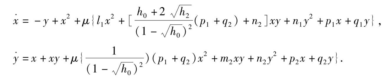
根据定理 3 可知,当 0 < | μ ≪1 |时,此系统在原点外围出现一个充分大的二重极限环,它是系统(17)经微扰系数后,从无限大分界线跳出来的.
致谢:作者对陈孝秋同志曾指出本文初稿中计算上的问题,并给予指正表示感谢!
参考文献
[1]陈孝秋.一类二次系统存在 Poincare 分支的条件,汕头大学学报,1987,2 (1 ):12-16.
[2]叶彦谦等.极限环论.上海:上海科学技术出版社,1984,83-88.
Abstract : In this paper we use the Poincare bifurcation theory to prove that there may be just one double limit cycle or just two single limit cycles jumping out of the periodic cycle region in a quadratic system, and that there may be just one double limit cycle or just two single limit cycles jumping from an infinite separatrix cycle with only one infinite critical point in a quadratic system. And we give respective specific examples for them.