下载掌阅APP,畅读海量书库
立即打开


Probability theory [1] is a discipline that uses mathematical methods to analyze random phenomena.Random phenomena are characterized by none certain regularity,but with some statistical regularity.If all possible results of a physical experiment or an imaginary experiment are known in advance,although the result cannot be determined before each experiment,it is known that the result must be one of the possible results,and the test can be repeated under the same conditions,then such experiment is called random experiment E .Each possible result is called basic event (also called sample point),denoted by the symbol ω .Basic events must be mutually exclusive.The set of all possible results of a random experiment is called basic event space (also called sample space),which is often represented by the symbol Ω .
In practice,ones may be more concerned about the probability that the experiment result is located in a certain domain within the sample space.For example,in the experiment of tossing a dice,the way to ask the question may be “how likely is it that the number of points is less than 5”.In order to describe such problems,we need to introduce the concept of events.A set of several basic events is called event .Thus,if the basic event space Ω is regarded as the universal set,then an event A should be a subset of Ω .After a random experiment,if the test result is a basic event in A ,then we say the event A happens.For example,if A represents an event that the point number of a dice is less than 5,then A ={1,2,3,4}.After tossing the dice,if the point is 3,we say A happens.Recall that the power set 2 Ω includes all subsets of Ω .Additionally,if the number of elements in Ω equals n ,then the number of elements in 2 Ω equals 2 n ,so there are totally 2 n events could be constructed based on the basic event space Ω .Among these events,there are two special events worth noting,one is the impossible event φ ,which does not contain any basic event,so it is impossible to occur.The other is the inevitable event Ω ,which contains all basic events,so it is inevitable to happen in the experiment.
Example 1.4.1 The following events exists in the experiment of tossing dice.
(1)The result is 1 ={1}.
(2)The result is even numbers ={2,4,6}.
(3)The result is even numbers less than 3 ={2}.
(4)The result is not even numbers ={1,3,5}.
(5)The result is not bigger than 4 ={1,2,3,4}.
With the above description,it is not difficult to find that basic events,basic event space and events can completely correspond to the concepts of elements,the universal set and subsets in set theory,as Table 1.4.1 shows.
Table 1.4.1 The correspondence of probability theory with set theory
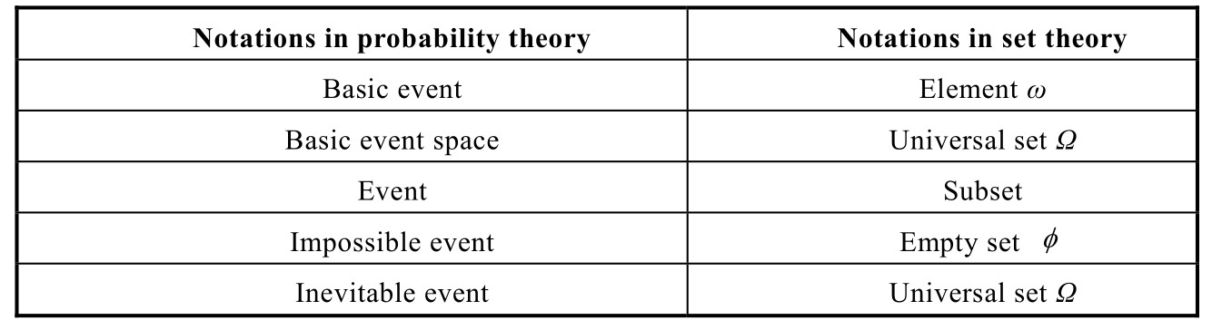
Because of such correspondence,we can view events from the viewpoints of set.All kinds of operations and properties in set theory can be applied into the analysis of event probability.The main task of probability theory is to analyze or calculate the probability of each event in a random experiment.However,for discrete sets and continuous sets,ones have to adopt different calculation methods,so it is necessary to classify the random experiments into discrete experiments and continuous experiments according to the type of basic event space.
Definition 1.4.1 A random experiment with basic event space being a finite or countable set is called discreate random experiment .A random experiment with basic event space being an uncountable set is called continuous random experiment .
If the basic event space is a finite set,it is called elementary probability theory.The probability distribution of discrete random experiment could be listed by a table.
Example 1.4.2
(1)The probability distribution for the experiment of tossing a dice is as follows.

(2)In a shooting practice,assume the probability of hitting and missing is p and q =1- p ,respectively.Keep shooting until it is hit.Use i to denote the number of shoots.Let ω i denote the basic event of shooting i times.Then the probability distribution is as follows.In this experiment,the basic event space is a countable set.

Definition 1.4.2 The probability that B occurs given that A has occurred is called the conditional probability and is denoted by P ( B | A ).
Definition 1.4.3 If P ( A )>0,then
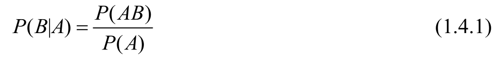
In many experiments,it may exist that the occurrence of event A has no impact on event B ,and vice versa.The occurrence of event A cannot provide any information to event B (thus does not change the probability of B ).If this is the case,the two events A and B are called independent of each other.In this case,the conditional probability P ( B | A )equals P ( B ),i.e.,
P ( B | A )= P ( B )or P ( AB )= P ( A ) P ( B ),given that A and B are independent.
Example 1.4.3
(1)Randomly taking an apple out from a bag,use W to denote its weight.
(2)Randomly choosing a student in a class,use H and X to denote his/her weight and age,respectively.
(3)In the shooting experiment,assume it will not miss the target.Use R to denote the distance between the hitting point and the target center.
(4)Tossing two dices,use S to denote the sum of their points.
In these examples,variables W , H , X , R and S have some common characteristics.On the one hand,they all represent some characteristics of the sample point(weight,height,age,distance,etc.),and their values change with the sample point,so these variables can be regarded as the functions of sample points(i.e.,functions with the sample space Ω as the definition domain).On the other hand,before the random experiment,one cannot determine the values of these variables.Only when the experiment is finished and the results(i.e.sample points)have been generated,we can know the values of these variables,so the values of these variables also show randomness.Such variables are called random variables.
Definition 1.4.4 The real-valued functions defined on the sample space are known as random variables .
According to the different types of the value range,random variables can be divided into two types.
(1)Discrete random variable:It can take only finite or countable values,that is,the value range of the variables is a discrete set.
(2)Continuous random variable:It can take uncountable values,that is,the value range of the variables is a continuous set.
In Example 1.4.3, X and S are discrete random variables,and W , H and R are continuous random variables.It can be seen that the classification of the two types of random variables is not based on whether the random experiment(or sample space)is discrete or continuous.In Example 1.4.3, W and H are based on discrete sample space,but they are continuous random variables.
The probability distribution of random variables in their range is a very important problem.The word “distribution”,as it literally means,describes the distribution of something in a certain area.The probability distribution of a random variable reflects the distribution of probability in the value range.
A discrete random variable X takes values from finite sets or countable sets,so the probability distribution can be listed in the form of Table 1.4.2 or Figure 1.4.1.Generally, p ( x )= P ( X = x )is called the probability mass function of the discrete random variable X .
Table 1.4.2 Probability distribution of a discrete random variable

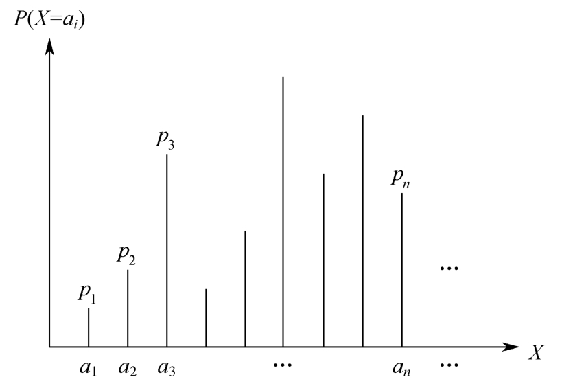
Figure 1.4.1 Probability distribution of a discrete random variable
A continuous random variable takes value from uncountable set(or continuous interval),so its probability distribution is a continuous function.In this case,it is meaningless to discuss the probability of P ( X = x ).What meaningful is the probability that X lies in a certain interval( c , d ),i.e., P ( c < X < d ),as Figure 1.4.2 shows.The continuous function curve f X ( x )plays similar roles to the discrete probability distribution in Figure 1.4.1.It clearly reflects the probability distribution of random variables in each interval within the value range,just like the density in physics,so it is called probability density function(PDF).The integral of f X ( x )in a certain interval equals the probability that the random variable X is located in the interval,so from Figure 1.4.2 ones get

Since the total probability is 1,the following normalization property must keep for any probability distribution.
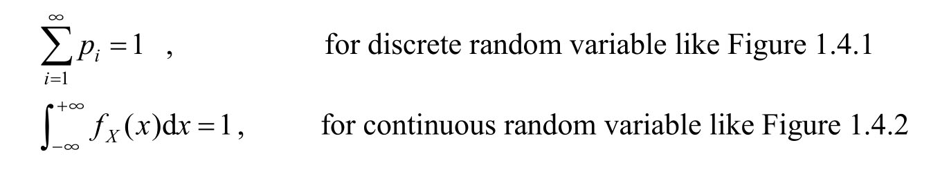
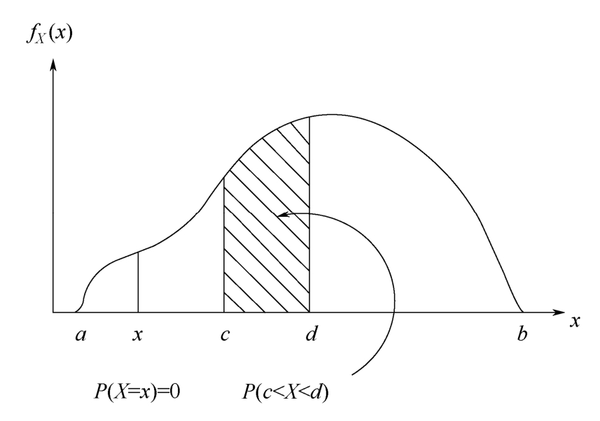
Figure 1.4.2 Probability distribution of a continuous random variable
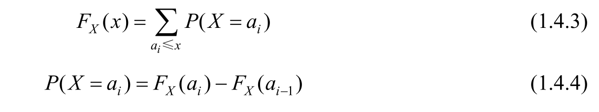
Definition 1.4.5 The function F X ( x )= P ( X ≤ x )is called the cumulative distribution function (CDF)of the random variable X .
Cumulative distribution function and probability distribution function could mutually convert into each other.Specifically,for a discrete random variable,we have
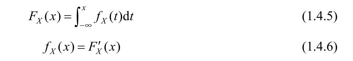
For a continuous random variable,we have
In practice,five discrete distributions and three continuous distributions are commonly used.
1.Bernoulli distribution
It is also called(0-1)distribution.The prototype of the physical experiment is a coin tossing experiment,with one side marked as X =0,and the other side marked as X =1.The probability distribution is listed in Table 1.4.3 and shown in Figure 1.4.3.
Table 1.4.3 Bernoulli distribution

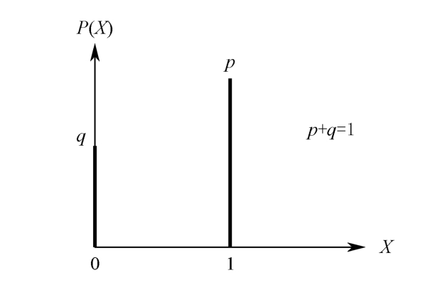
Figure 1.4.3 Bernoulli distribution
2.Binomial distribution
In a single shooting experiment,suppose the probability of success(hit)is p ,and the probability of failure(miss)is q =1- p .If the shooting is carried out n times independently,let X denote the times of success,then it is not difficult to calculate the probability of P ( X = k ).

X is called a binomial random variable,denoted by B( n , p ).Its probability distribution is listed in Table 1.4.4 and shown in Figure 1.4.4.
Table 1.4.4 Binomial distribution

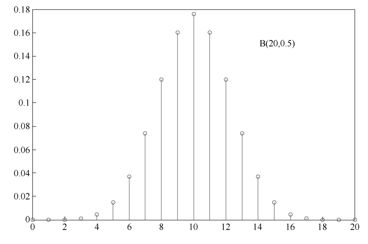
Figure 1.4.4 Binomial distribution
3.Geometric distribution
In the similar shooting experiment as above,if ones keep shooting until it is hit and use X to denote the times of shooting,then X is called a geometric random variable. P ( X = n )= q n -1 p .Its probability distribution is listed in Table 1.4.5 and shown in Figure 1.4.5.
Table 1.4.5 Geometric distribution

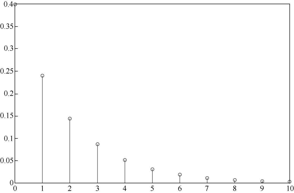
Figure 1.4.5 Geometric distribution
4.Hypergeometric distribution
Assume there are N balls with the same shape in a bag,including M red balls and N - M black balls.Randomly take out n balls from the bag,and use X to represent the number of red balls,then the probability distribution of X is

X is called a hypergeometric random variable,denoted by X ~ H( n , N , M ).The probability distribution with parameters N =100, M =10, n =20 is as Figure 1.4.6 shows.
5.Poisson distribution
A random variable X ,taking one of the values from 0,1,2,…,is said to be a Poisson random variable with parameter λ if for some λ >0.

A Poisson distribution with parameter λ = 5 is shown in Figure 1.4.7.
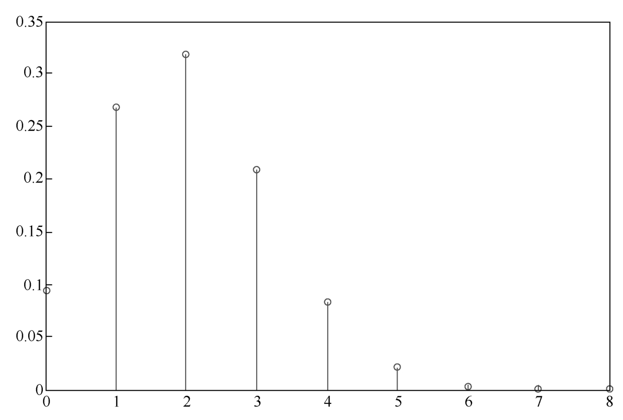
Figure 1.4.6 Hypergeometric distribution
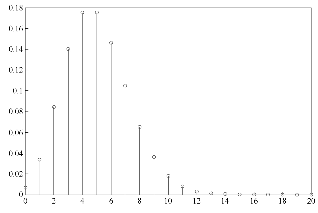
Figure 1.4.7 Poisson distribution
6.Uniform distributio n
A point uniformly lies in the interval [ a , b ],and the coordinate of the point is expressed by the random variable X ,then it is a uniform distribution random variable.The probability interpretation of the word “uniform” is that the probability density function f X ( x )is constant in the value range.For the random variable X uniformly distributed in the interval [ a , b ],it is often denoted by X ~U[ a , b ].Its distribution is shown in Figure 1.4.8 and its probability density function is
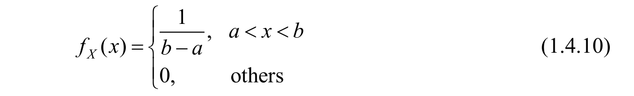
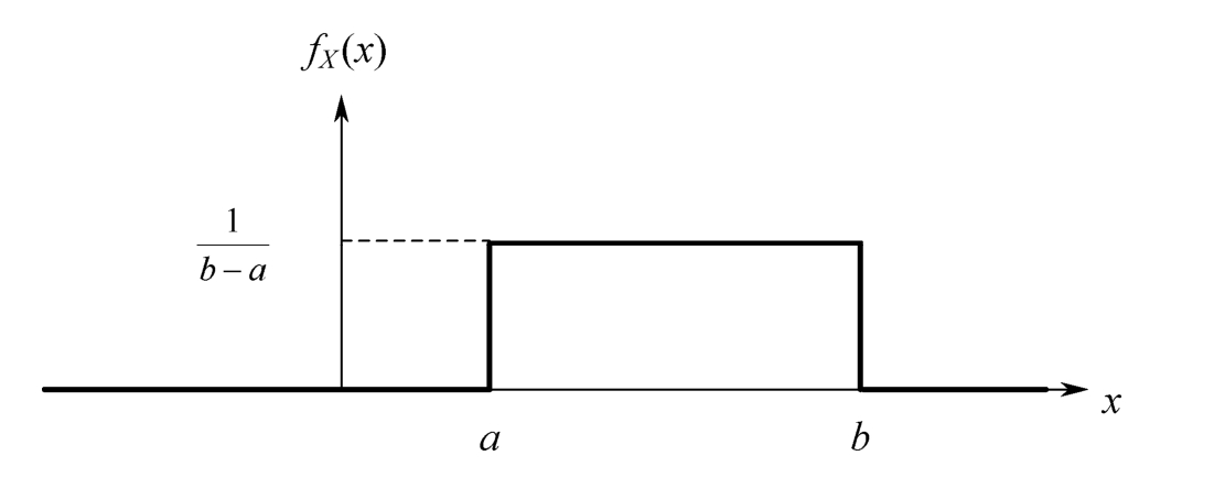
Figure 1.4.8 Uniform distribution
7.Exponential distribution
A random variable X is governed by exponential distribution if it has the following probability distribution.Taking λ = 1 as an example,the probability distribution is shown in Figure 1.4.9.
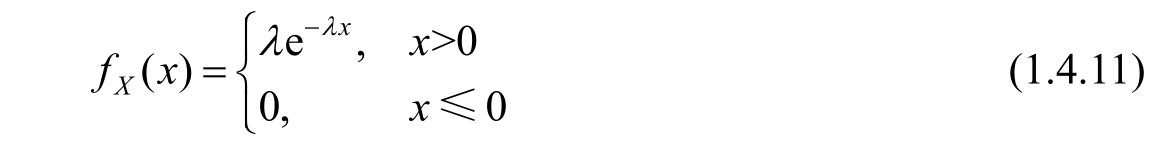
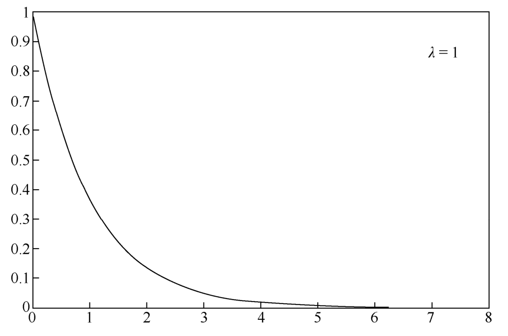
Figure 1.4.9 Exponential distribution
8.Normal distribution
We say that X is a normal random variable,in short, X is normally distributed,with parameters μ and σ 2 if the probability density function of X is given by
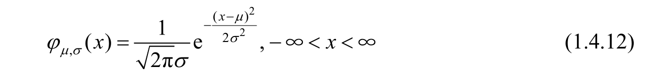
Normal distribution is always called Gaussian distribution in engineering,which is denoted by X ~ N( μ , σ 2 ).Especially,if μ =0 and σ 2 =1,then it is called the standard normal distribution,which is shown in Figure 1.4.10.
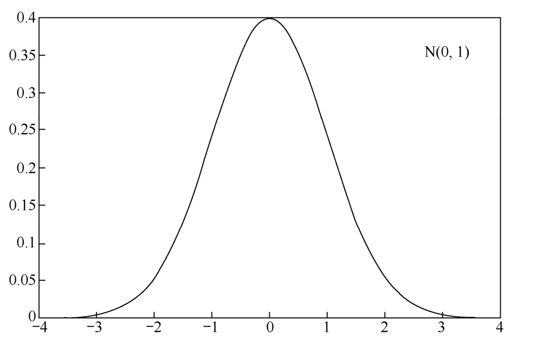
Figure 1.4.10 Standard normal distribution
The cumulative distribution function and probability distribution function are accurate and complete description of the probability distribution of the random variables.However,many practical problems do not need to know(sometimes cannot know)such a detailed description of the probability distribution,but only need to know some basic characteristics,such as the average score of students in a class and the fluctuation of students' scores near this average value,which requires the concept of numerical characteristics of random variables.
Definition 1.4.6 Assume the probability distribution of a discrete random variable X is like
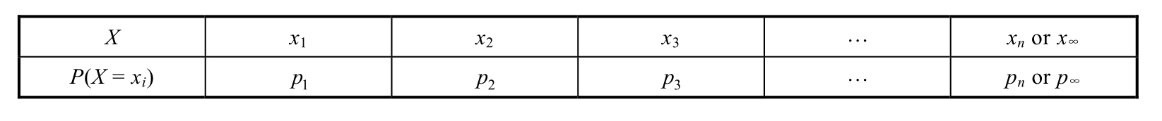
Then the expectation of X ,denoted by E ( X ),is defined by

Assume a continuous random variable X has the probability density function of f X ( x ),then the expectation of X is defined by

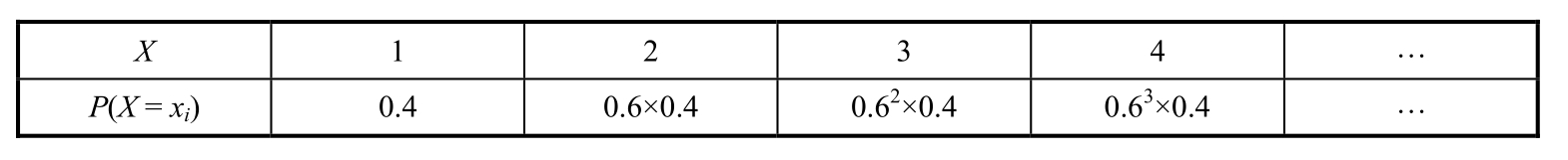
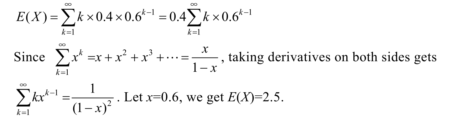
Example 1.4.4 There are 2 white balls and 3 black balls in the bag.Take out a ball and watch its color,if it is black,put it back to the bag and make next trial.The trial continues until a white ball is taken out.Use X to indicate the number of times for the trials.Calculate the expectation of X .Obviously, X is a geometric random variable with parameters p =0.4 and q =1- p =0.6.
The probability distribution of X is as
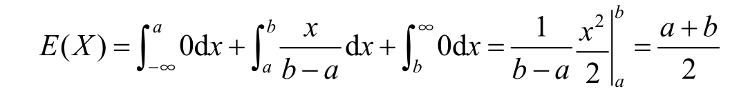
Example 1.4.5 A continuous random variable X uniformly distributed over the interval [ a , b ].So the probability density function of X should be
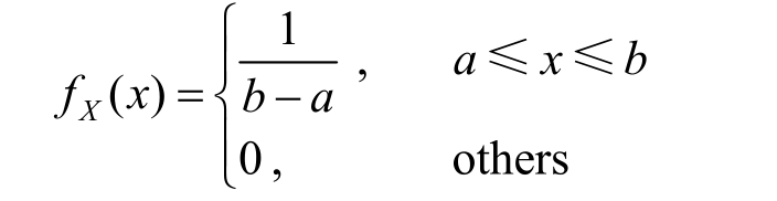
Then we have
Theorem 1.4.1 X is a random variable and Y = g ( X )is a function of X ,so Y is a new random variable yet.Then the expectation of Y could be computed by
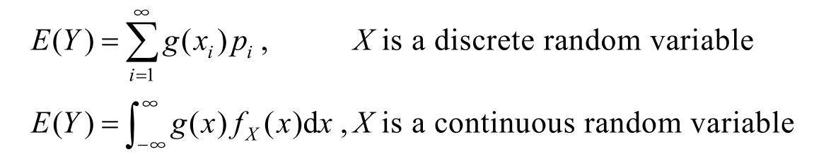
Definition 1.4.7 X is a continuous random variable.The expectations of following functions of X are called moment .
(1) g ( X )= X k , k ≥0

(2) g ( X )=|X| k , k ≥0

(3) g ( X )=( X - E ( X )) k , k ≥0

(4) g ( X )=|X-E(X)| k , k ≥0
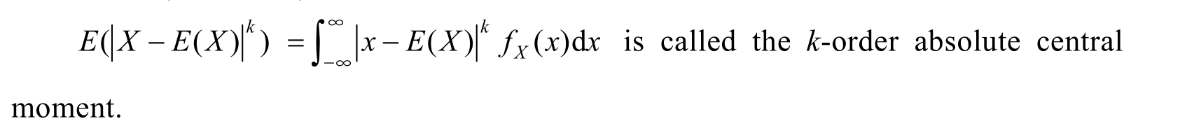
If X is a discrete random variable,the definition is similar,only need to change the operation from integral to sum.2-order central moment is the most important one among all moments.It is also called variance.
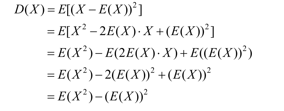
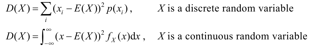
Definition 1.4.8 If X is a random variable with the expectation E ( X ),then the variance of X ,denoted by D ( X ),is defined by

Specifically,
A more common calculation of D ( X )is given below.