
下载掌阅APP,畅读海量书库
立即打开


 用于移植的朗格汉斯岛(胰岛)的分离
托马斯等
编者按
本文介绍了一种用于分离大鼠朗格汉斯岛(胰岛)的方法,以用作治疗糖尿病的潜在移植来源。通过移植整个胰腺治疗糖尿病的尝试收效甚微,而分离产生胰岛素的胰岛的尝试受到了方法学问题和低生存力的限制。由托马斯和他的同事在英国谢菲尔德所改良的方法,获得了大量可存活的胰岛,这种方法包含消化、洗涤和分离几个步骤。现在胰岛细胞移植正被评估是否可作为一种治疗I型糖尿病的潜在方法,在I型糖尿病中,免疫系统会破坏产生胰岛素的胰岛β细胞。成功的移植可以减少或消除对胰岛素治疗的依赖。 英文
迄今为止,胰腺移植用于治疗糖尿病成效甚微。1971年,经过这样治疗并在移植登记处登记备案的23例患者中 [1] ,有15例在3个月内死亡,生存时间最长的患者也只有1年。一个主要的问题就是患者在移植前需要克服胰腺外分泌消化和胰管结扎(“班廷胰腺”)。但是,德拉格施泰特 [2] 发现,经过这样治疗的狗在数月后会患糖尿病或者表现出糖尿病糖耐量试验的结果,这很可能是由于胰岛的纤维化以及继发的贫血造成的。伴血液供应的全腺体移植是目前的主流,但是伴随免疫排斥发生的血栓、渗漏和消化等问题使得该方法到目前为止也没能取得成功。 英文
人们试图从胰腺中分离出胰岛以研究葡萄糖代谢。赫勒斯特伦 [3] 描述了一种显微解剖技术,但是这种方法非常繁冗,而且只能得到少数的胰岛细胞团。此后,莫斯卡勒夫斯基 [4] 描述了一种胶原酶消化法,该法已经在兔子中取得成功,而且分离出的胰岛数量也得到提高,后来莱西和科斯蒂安诺夫斯基 [5] 在大鼠中对这个方法进行了改进。但是,即便使用了诸如区带离心和密度梯度离心的分离方法,仍然很难获得游离的胰岛,而且这些细胞的生存能力也是一个大问题。 英文
我们建立了一种方法,并用此法从大鼠胰腺中稳定制备了大量用于移植的胰岛,并且通过移植确认了细胞的生存能力。 英文
起初使用的是白化的远交系大鼠,后来使用年轻成年的头部有斑点的顶罩大鼠(PVG/C系)的近交系。颈椎脱臼法处死大鼠后,刮除腹面毛发,用溶于酒精的氯己定处理后选取正中线切口开腹。使用解剖显微镜放大10倍,将一条细小的聚乙烯导管(“Intracath”(译者注:一种留置针)—巴德,伦敦)插入胆总管,并用2–0的亚麻缝合线固定。在导管恰好进入十二指肠前,用动脉钳夹闭其下端。注射10 ml含有2 mg·ml –1 牛血清蛋白(第五组分)的汉克氏液(译者注:一种用于细胞培养的平衡盐溶液)使胰腺膨胀。经过一些实践之后我们发现,这些步骤可以在动物死后5分钟之内完成。将胰腺摘除并转移到一个玻璃培养皿内,用剪刀将其剪碎并去除所有多余的脂肪。然后将其转移到一个试管内,并加入10 ml的汉克氏液。胰腺组织沉到管底,所有残存的脂肪都会漂浮在表面,将它们吸出并丢弃。将制备好的组织转移到一个小的锥形瓶内,该瓶内装有2 ml含0.6 mg·ml –1 葡萄糖和I型胶原酶(西格玛化学公司,伦敦)的汉克氏液。把盖好的瓶子置于37℃水浴摇床内约30分钟。分离过程的限速步骤是解剖显微镜下的频繁取样和检查。 英文
将消化好的胰腺转移到一个试管内,用含有相同浓度葡萄糖的冷的汉克氏液稀释,温和离心1分钟。弃上清液并加入新鲜的培养液(汉克氏液),得到的悬浮液过滤到培养皿内;该培养皿的底为暗色,以便于在放大10倍的解剖显微镜下进行观察。 英文
起初,许多细小的腺泡组织碎片使得视野很模糊;轻轻地摇动培养皿使其悬浮在汉克氏液中,然后将其吸出并丢弃,而胰岛则存留在容器底部。通过暗场照明能够清晰地看到它们呈黄白色的圆顶状(图1),用尖端拉长的巴斯德吸管将其移出。图2显示了分离出来的胰岛的组织学形态。其结构和细胞表现正常。 英文

图1. 通过暗场照明观察到的从胰腺中分离出来的胰岛细胞组织。解剖显微镜下放大5倍。

图2. 分离出的胰岛。正常的结构和细胞外观。苏木精—伊红染色,放大300倍。
用这种方法能够在每个大鼠胰腺中得到多达350个胰岛。为了获得更多胰岛,大鼠胰腺以四个为一组一起处理。 英文
将分离的胰岛细胞移植到同种大鼠的肾小囊内或者睾丸内以确认其生存能力。最长的随访期是1个月,此时可以观察到成活的胰岛细胞含有能被醛复红染色的β细胞颗粒。同样的方法在兔子中也获得了成功。 英文
1889年,冯·梅灵和明科夫斯基阐述了胰岛和糖尿病之间的关系 [6] 。1892年,埃东 [7] 证明了移植到皮下的一小块胰腺可以延缓进行胰腺切除术后的动物出现糖尿病症状。在大量有关胰腺移植的文献中,人们都忽略了胰岛细胞移植的想法,尽管有一篇早期报道提出移植的胰岛可能会减轻在大鼠中由四氧嘧啶诱导的糖尿病 [8] 。 英文
现在,我们已经在近交的免疫同系的动物品系中成功地建立了一种分离胰岛的方法,这使得移植研究摆脱排斥问题的困扰成为可能。正如在对胰岛细胞的生存力研究中所证实的,这些细胞能够被移植并能生存相当长的时间。胰岛细胞移植的组织学和功能方面的研究将另作报道。 英文
我们感谢联合谢菲尔德医院的捐助基金和医学研究理事会的资金。我们感谢劳伦斯·亨利博士帮助进行组织学检查,感谢滕斯蒂尔先生及其职员在成像方面的帮助。 英文
(毛晨晖 翻译;王敏康 审稿)
Seismic Travel Time Evidence for Lateral Inhomogeneity in the Deep Mantle
B. R. Julian and M. K. Sengupta
Editor’s Note
The Earth’s lower mantle is inaccessible for direct study. The best method for probing it is through the measurement of seismic waves, which travel at different speeds through materials of different density or composition. Although there were some earlier signs that the lower mantle is not uniform but somehow “lumpy”, Bruce Julian and Mrinal Sengupta at the Massachusetts Institute of Technology here provide clear evidence from seismic travel times that the lowest part of the mantle is inhomogeneous on scales of around 1,000 km. They could not offer definitive reasons, but suggest that at least some of the irregularities might be caused by convection structures: specifically, by plumes of rising, hot material, which others had proposed earlier. 中文

We present evidence from seismic travel time data of lateral variations in the properties of the lower mantle. The size of some anomalies is about 1,000 km. 中文

EVIDENCE from seismic body wave and surface wave data has long indicated that the Earth’s upper mantle (depth <700 km) is strongly laterally heterogeneous. Lateral variations of the compressional wave velocity as large as 10% have been reported for the upper 200 km, and the shear velocity probably varies even more. For depths greater than 700 km, however, the existence of lateral variations has been more difficult to establish, although such variations have been invoked by various workers 1,2 to explain the scatter of some seismological data. Greenfield and Sheppard 3 , in a study of d T /d∆ measurements made at the Large Aperture Seismic Array in Montana, found a pronounced difference between data from events to the northwest and the southeast for epicentral distances greater than 60°, which could not be attributed to the structure beneath the array, and seems explicable only in terms of heterogeneities in the lower mantle. Davies and Sheppard 4 have presented a more extensive collection of data of this type in the form of an “array diagram”, on which d T /d∆ and azimuth anomalies are represented as vectors in slowness space. Many anomalies are found which are too large to be effects of upper mantle heterogeneities in the source regions; on the other hand, the anomalies often vary rapidly with the direction of approach of the waves, implying that structure directly beneath the array is not responsible. Further evidence has come from a study of the diffraction of compressional waves by the Earth’s core, in which Alexander and Phinney 5 found that the region of the core-mantle boundary beneath the Pacific Basin is distinctly different from the region beneath the North Atlantic and Africa. 中文
We have found evidence that significant lateral variations occur in the lowest few hundred km of the mantle, this region being much more heterogeneous than that which lies above it. The methods of this travel time study are described in detail elsewhere 6 . 中文
We restricted the study to data from deep focus earthquakes in an attempt to avoid systematic errors caused by near source velocity variations in the upper mantle, which are particularly severe in seismically active regions. About 3,300 arrival time data from 47 earthquakes with depths between 450 and 650 km were used, all events being located in the deepest parts of their respective seismic zones. For most of the 18 seismic regions involved, two or more events were available, and for each station a consistency check was made to eliminate data contaminated by gross errors. An iterative procedure, similar to the one described by Herrin et al. 7 , was then used to determine the earthquake locations, the travel time curve for a 550 km focal depth, and a set of “station corrections”(each represented by a constant) to account for the effect of lateral variations in the upper mantle beneath the stations. 中文
The travel time curve thus determined is shown in Fig. 1 (in terms of deviation from the standard Jeffreys-Bullen tables), together with the data means and their standard errors for 2°distance intervals. This curve is similar in shape to those found in other recent studies 7,8 except beyond 85°, where most other curves remain approximately parallel to the Jeffreys-Bullen curve, but ours becomes progressively earlier by about 0.9 s. Fig. 2 shows some of the data which have contributed to the determination of the travel time curve; the observed times show a striking dependence upon the location of the earthquakes. The difference between the curves in Fig. 1 results from differences in the geographic regions sampled. Possible causes of a regional dependence of this nature are velocity variations in the upper mantle in the source or receiver regions or in the lower mantle, and mislocation of the events (caused by uneven station distribution, and so on). Event mislocation and structure in the receiver regions can be ruled out because they would be expected to produce similar effects at all epicentral distances. Although the observed variations are most striking beyond 85°, we shall show that they are much smaller at distances less than 70°. It is conceivable that structure in the source regions could produce a distance dependent regional variation of this kind, if the velocity anomalies were systematically located relative to the earthquake hypocentres (as indeed they are beneath island arcs). In that case the variations would have to be localized in a very small region beneath the hypocentres, because a 10° distance interval maps into about a 5° difference in angle at the focus. Even if the anomalous regions are as deep as 1,000 km, the velocity change must occur over a horizontal distance of only 50 km or so. This possibility may be ruled out because all the earthquakes in each source region yield a similar pattern of travel time residuals, even though the epicentre locations in each region are typically distributed over >200 km. Velocity variations near the focus are further ruled out because early arrivals beyond 85° are not restricted to observations of deep earthquakes; they also occur, for example, in data from nuclear explosions in the Marshall Islands 9 . 中文

Fig. 1. P wave travel time curve (focal depth 550 km) determined in this study (——), expressed in terms of deviations from the Jeffreys-Bullen values. Data means and their standard errors are indicated for 2° distance intervals. Surface focus curves of Herrin et al. 7 (——) and Lilwal and Douglas 8 (---) have been displaced vertically for ease of comparison.
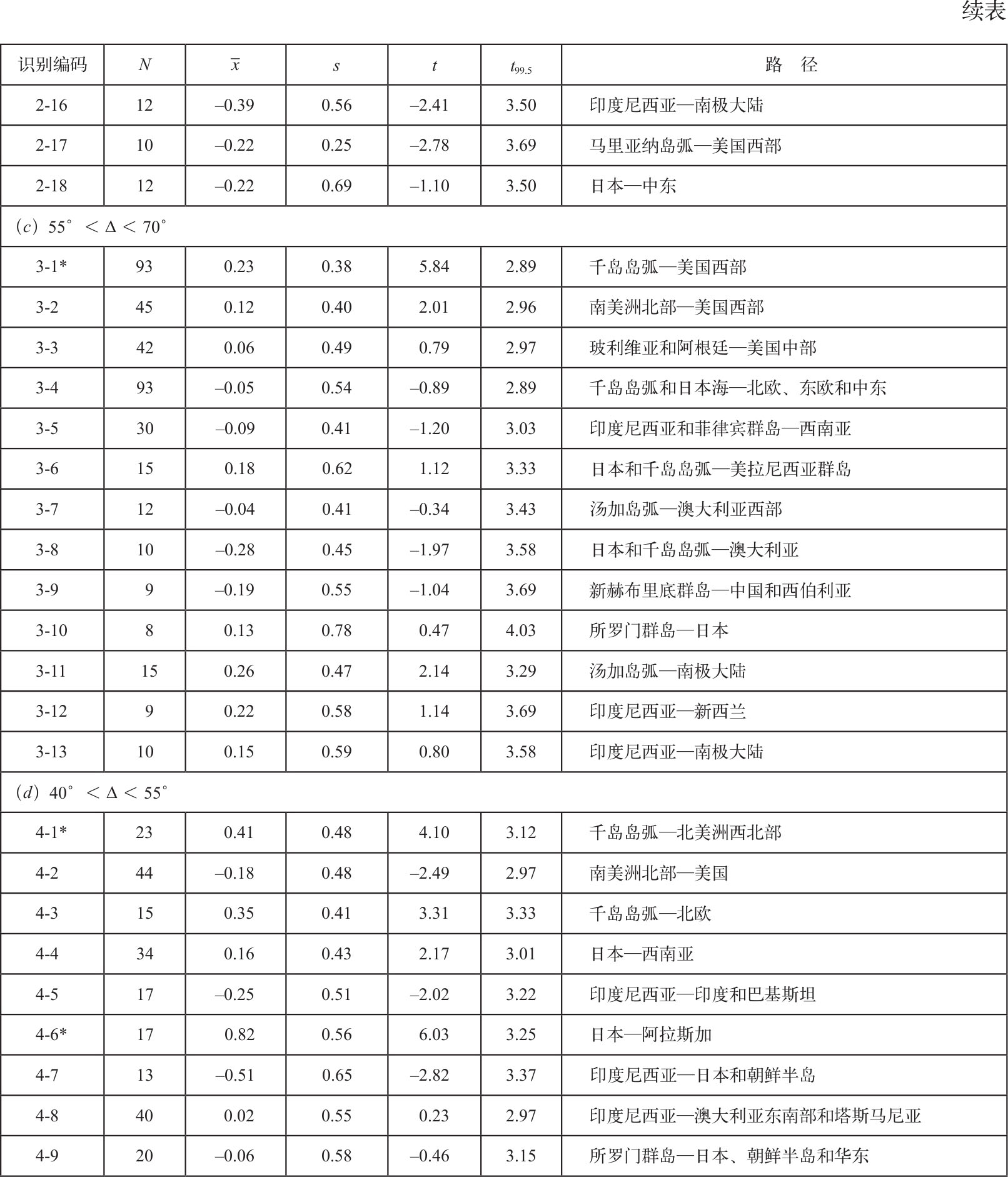
It seems, then, that lateral variations of compressional velocity in the middle or lower mantle are required to explain the travel time anomalies. But because of the uneven distribution to seismological observatories and deep earthquakes, the sampling of the mantle provided by available data is uneven, and it is impossible to determine uniquely the complete three dimensional velocity structure of the mantle. What can be determined is the average travel time residual for each of a number of “bundles” of rays following nearly identical paths from a seismic region to a group of stations, and from this information we infer the most probable cause of the variations. Table 1 summarizes the travel time data for all paths for which 9 or more observations are available. For each path a Student’s t test has been used to evaluate the hypothesis that the mean travel time (after station corrections have been applied) is the value given by the curve in Fig. 1 and that deviations from this curve can be attributed to random measuring errors. Those ray paths for which the hypothesis could be rejected at the 99.5% confidence level are indicated in Table 1. Fig. 3 shows histograms of the residual distribution for these anomalous paths. For observations at distances beyond 70°, 16 paths (out of 34 tested) showed significant variations from the average curve, whereas for smaller distances, only 3 anomalous paths (out of 22) were found. This strongly suggests that most of the scatter originates in the deep mantle (depth >2,000 km). The possibility of the variations occurring at a shallower depth cannot be absolutely disproved, but the velocity distribution in the Earth would have to be such that, given the distribution of earthquakes and seismic stations, all observed waves bottoming at the depth of the heterogeneities happen to be unaffected by them (even though P waves spend about 25% of their travel time traversing the lowest 10% of the ray path), while waves penetrating beneath the heterogeneities are affected. It seems unreasonable to assume such a conspiratorial behaviour on the part of the velocity variations when a much simpler hypothesis is available. 中文

Fig. 2. Travel time data (with station corrections applied) for earthquakes in ( a ) the Sea of Okhotsk and ( b ) Argentina. The solid line is the curve derived from all data.
Table 1. Travel Time Statistics for Mantle P Wave Paths


N =Number of observations.
 =Mean travel time residual after station correction (s).
s =Standard deviation of residuals (s).
t
=

t 99.5 =99.5% confidence limit for | t | if true mean is zero.
* Indicates paths with mean significantly different from zero.

Fig. 3. Histograms of travel time residuals (relative to curve of Fig. 1 with station corrections applied) for different ray paths through the mantle. Identification numbers correspond to those in Table 1 and Fig. 4. N is the number of observations.
The actual details of the velocity distribution cannot, however, be determined precisely, because rays travel a great distance at approximately the same depth near their turning points. Fig. 4 shows the regions of the lower mantle sampled by the various ray bundles (defined arbitrarily as the central 30°of each path) and indicates which paths correspond to early and late arrivals. These are in most cases probably the regions where the actual velocity anomalies occur. Where regions overlap on the figure, they are generally consistent with each other (for example, regions 1-6 and 1-7, regions 2-2 and 2-3, and regions 4-1 and 4-6). This consistency is encouraging, in that it supports our argument that the travel time anomalies originate in the deep mantle and are not the result of some other type of systematic error. An apparent inconsistency exists between regions 1-3 and 1-16, but this is not surprising because of the uncertainty as to exactly where the travel time anomalies actually originate. The rays following path 1-3 also pass through regions 2-2 and 2-3 further to the north, and it is likely that the travel time anomaly actually originates there. Another interesting feature of Fig. 4 is a correlation between the anomalies in the two greatest distance ranges (for example, regions 1-7 and 2-7, regions 1-4 and 2-4, and regions 1-5 and 2-6), suggesting that the structure in the deep mantle has a spatial “coherence” of at least a few hundred km vertically. 中文

Fig. 4. Regions where paths of observed P waves bottom in the mantle. Cross-hatching indicates regions differing significantly from the mean determined from all data. Other regions tested are outlined. The identification numbers correspond to those in Table 1 and Fig. 3.
 Late;
Late;
 , Early.
The mean travel times in Table 1 show a variation of about 1.5 s for rays bottoming below 2,600 km, and about 0.6 s for rays bottoming between 2,000 and 2,600 km. These numbers are somewhat uncertain, but it is likely that the true travel times vary by at least 1 s. The amount by which the actual velocity in the mantle varies depends on the size of the regions within which the variations occur. The data of Fig. 4 suggest that the size of some of the anomalies, at least, is about 1,000 km or less, in which case the velocity must vary by at least 1%. This is a lower bound both because we have probably overestimated the scale of the inhomogeneities and because we are measuring averages of the velocity in rather large regions and some cancellation of the effects of positive and negative velocity anomalies is likely. Combined interpretation of travel time and d T /d∆ measurements can probably improve the resolution of structural details. 中文
Might the deep mantle variations be related in some way to the convection plumes hypothesized by Wilson 10 and Morgan 11 to exist in the deep mantle? To answer this the region of the Hawaiian Islands provides the best data, and here they indeed indicate a pronounced lateral variation, the velocities being high to the northwest of Hawaii (regions 2-2, 2-3, and probably 1-3) and low in the vicinity of the islands (regions 1-4, 2-4, and 1-6). Interestingly, the d T /d∆ data presented by Davies and Sheppard 4 also indicate a horizontal velocity contrast of this sort in the vicinity of Hawaii. Unfortunately, no other proposed plumes are well sampled by our data. Region 1-13 includes the Mascarene Islands, but the data here are highly scattered, and no conclusion can be drawn. Regions 1-5 and 2-6, both with apparently high velocities, are located slightly to the northeast of the Galapagos Islands, so it is not clear what relation, if any, this velocity anomaly may bear to a possible plume. If travel time data for rays passing through more proposed plume regions can be obtained, they may provide valuable evidence relevant to the Wilson-Morgan hypothesis. 中文
Except, perhaps, for the Hawaiian Islands, no geological or tectonic features show an obvious correlation with the inferred deep mantle velocity anomalies. At shallower depths, however, this is not the case; regions 3-1, 4-1, and 4-6, all seeming to have low velocities, lie beneath the Kurile and Aleutian Island arcs. The only other island arc adequately sampled at these depths lies beneath Middle America (region 4-2) and is associated with early arrivals (though they are not significant at the 99.5% confidence level). The data thus suggest that low velocities may be characteristic of island arcs at depths greater than 1,000 km. 中文
The data considered here do not support any correlation between velocity variations below 2,000 km and global gravity anomalies or geoid heights. At shallower depths such a correlation does exist, but it is merely another manifestation of the low velocities beneath the Kurile and Aleutian Islands, because the concave sides of island arcs are generally the sites of prominent positive free air gravity anomalies. 中文
It is not possible to make a direct comparison between these results and those of Alexander and Phinney 5 . The region of the North Atlantic found by them to be anomalous is further east than the corresponding region sampled by our data. Further, travel time measurements such as ours provide a measure of the average velocity in a region, whereas the behaviour of core diffracted waves depends on features such as the velocity gradient in the lower mantle. Further studies of variations in the “visibility” within the core shadow would be a useful complement to travel time and d T /d∆ studies of the lower mantle. 中文
We thank Dr. David Davies and Dr. M. Nafi Toksöz for helpful suggestions. This work was sponsored by the Advanced Research Projects Agency of the Department of Defense. 中文
( 242 , 443-447; 1973)
Bruce R. Julian and Mrinal K. Sengupta
Lincoln Laboratory, Massachusetts Institute of Technology, Lexington, Massachusetts 02173
Received January 2, 1973.
References:
深地幔横向非均匀性的地震波走时证据
朱利安,森古普塔
编者按
对地球的下地幔是无法进行直接研究的。探测下地幔的最好方法是测量地震波,因为在不同密度或不同组分的岩层中,地震波传播速度会有所不同。早前已有一些迹象表明下地幔不是均一的并且多少呈“块状分布”,本文中,麻省理工学院的布鲁斯·朱利安和姆里纳尔·森古普塔给出了确切的证据,他们从地震波走时的研究中发现,地幔最深处具有约1,000 km尺度范围的非均质体。他们没能给出确切的解释,但是他们提出,至少有部分非均质体可能是由对流结构所致:特别是受到了地幔柱上升、热物质的影响,这一点早前已有人提出。 英文
我们提供了来自地震波走时的、能表明下地幔物质存在横向变化的证据,一些异常体的尺度约为1,000 km。 英文
地震体波和表面波的数据早已证明,地球上地幔(深度<700 km)的横向不均匀性是非常突出的。有报告显示,在地幔上部200 km以内纵波速度的横向变化可达10%,而切变波速度的变幅可能更大。然而,在大于700 km的深处很难确定地震波的横向变化,不过还是有一些人 [1,2] 曾引用这种变化来解释某些地震数据的离散现象。在蒙大拿州的大孔径地震台阵测量d T /dΔ的研究中,格林菲尔德和谢泼德 [3] 从实验数据中发现,在西北和东南方向上震中距相差达60°以上,这不能归因于台阵下方的构造,似乎只能用下地幔的不均匀性来解释。戴维斯和谢泼德 [4] 以“阵列图”的形式广泛收集了这类数据。在这幅图中,d T /dΔ和方位角差异表示慢度空间矢量。图中显示出大量的异常,由于这些异常过大,因此不可能是震源区上地幔不均匀效应所致;另一方面,这些异常会随着地震波传播方向的改变而快速变化,表明这与台阵正下方的地质构造没有关系。而且对于由地核引起的压缩波衍射的研究进一步验证了上述观点,亚历山大和菲尼 [5] 发现,位于太平洋海盆下方的核幔边界区和位于北大西洋及非洲下方的核幔边界区迥然不同。 英文
我们已经发现,在地幔最底层的数百公里内,地震波的走时发生明显的横向变化,这一区域与其上方区域相比具有更大的不均匀性。这种基于走时的研究方法在另一篇文章 [6] 中已作详述。 英文
我们将研究范围限于深源地震,以避免上地幔中由近源速度变化引起的系统误差,而这种变化在地震活动区尤为强烈。我们选用了47次地震的3,300个到时数据,这些地震的震源深度在450 km至650 km之间,并且均位于各自所处地震带的最深处。所涉及的18个地震带中,大多都有两次或两次以上的地震数据是可用的。另外,为了消除含有过失误差的数据,每个台站的资料都进行了一致性检验。利用一种类似于赫林等人 [7] 所描述的迭代法,我们确定了地震位置、一条震源深度为550 km的地震波走时曲线和一组“台站校正量”(每个台站对应一个常数),每个常数代表走时在该台站下方上地幔的横向变化造成的影响。 英文
由此得出的走时曲线如图1所示(以相对于标准的杰弗里斯-布伦走时表的偏差表示),图中也显示了间距为2°的数据的平均值及其标准误差。在85°以下,曲线的形状与近期其他研究发表的曲线 [7,8] 相似,大部分其他曲线仍然与杰弗里斯-布伦曲线近似平行,但我们的结果逐渐提前了约0.9 s。图2显示了绘制走时曲线所使用的一些数据;观测到的走时大小很大程度上取决于地震发生的位置。图1中几条曲线的差异是由采样点的地理区域不同引起的。导致区域性差异的原因可能是源区或接收区上地幔地震波速度变化造成,或是由下地幔传播速度的变化引起,还可能是震源定位存在误差(由台站分布不均匀等原因造成)。震源定位的误差以及接收区的地质构造造成的影响可以排除,因为无论震中距大小,这两种因素所造成的影响是相似的。虽然在85°以上观测到的差异最为显著,但同时我们看到,在震中距小于70°时这种差异要小得多。如果传播速度的异常相对于震源呈系统性分布的话(在岛弧下方确实如此),那么可以推断,这种依赖于距离的区域差异是由震源区的地质构造引起的。如果是这样的话,距离的变化应该只局限在震源下方一个很小的区域,因为10°震中距间距可映射为震中处5°角度差。即使异常区深达1,000 km,速度变化肯定也只会发生在50 km左右的水平距离上。这种可能性应该可以排除,因为每一震源区内所有的地震都产生相类似的走时残差,即便在同一地震区内其震中位置的分布范围超过200 km也不例外。震源附近传播速度的差异也被进一步排除,因为在85°以上较早到达的地震波并不仅仅能在深源地震中观测到。例如,在马绍尔群岛的核爆炸数据中就出现过这种情况 [9] 。 英文
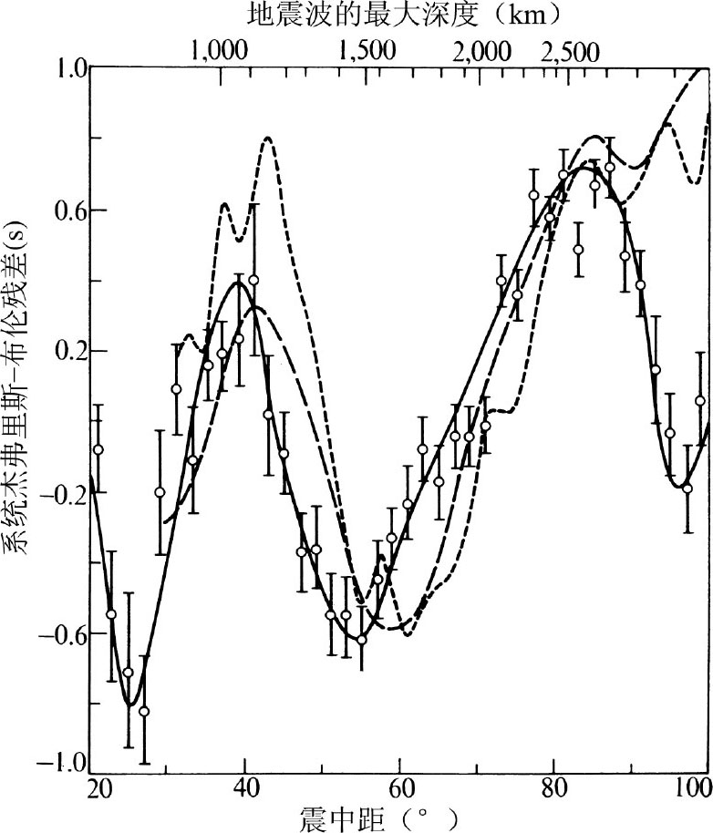
图1. 本项研究在震源深度550 km条件下得出的P波走时曲线(——),以相对于杰弗里斯-布伦走时表的偏差表示。数据平均值及其标准误差以2°的间距表示。为了便于对比,赫林等人 [7] (——)以及利尔沃和道格拉斯 [8] (---)的浅源地震曲线也垂直呈现于图中。
那么,似乎可以用纵波在中地幔或下地幔中传播速度的横向变化来解释走时的异常。但是,因为地震观测台站的分布不均匀且震源较深,所以现有数据提供的地幔采样也是不均匀的,因此也不可能确定地幔中完整的三维速度结构。对于每一组沿着近似相同的路径、从一个震区传播到一组接收台站的射线束,我们可以确定它的平均走时残差,根据残差信息我们可以推测造成这些差异最有可能的原因。表1总结了所有路径的走时数据,这些路径均有不少于9次的有效观测值。对每个路径应用学生 t 检验方法来检验下述假说:平均走时(经过台站校正以后)为图1中曲线给出的数值,并且相对这条曲线的偏差可以归因于随机测量误差。表1中对在99.5%的置信水平上背离上述假说的射线路径进行了标记。图3是这些异常路径的走时残差分布直方图。对于震中距超过70°的那些观测值,有16个路径(共检验了34个)显著偏离平均曲线;而对于震中距较小的那些观测,则只有3个异常路径(共检验了22个)。这有力地表明大部分散射产生于深地幔(深度>2,000 km)。在较浅处发生这种变化的可能性也不能绝对排除,但是如此一来,鉴于地震以及地震台站的分布情况,地球内部传播速度的分布就必须具有如下特点:观测到的底及非均质体底部的地震波恰巧未受到这些非均质体的影响(虽然P波在穿过最下方的10%的路径上消耗了近25%的走时),而穿过非均质体下方的地震波却受到了影响。当一个更简单的假设存在时,在速度变化上作这样一个特性诡秘的假设似乎并不合理。 英文
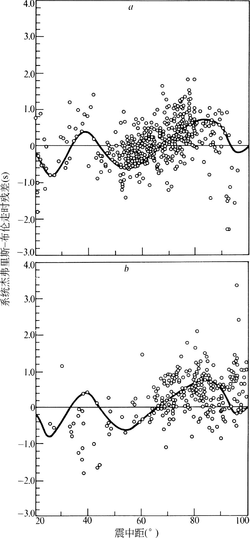
图2. 鄂霍次克海( a )和阿根廷( b )区域的地震波走时数据(已经过台站校正)。实线是由全部数据的拟合得到的。
表1. 地幔中P波沿各条路径走时的统计
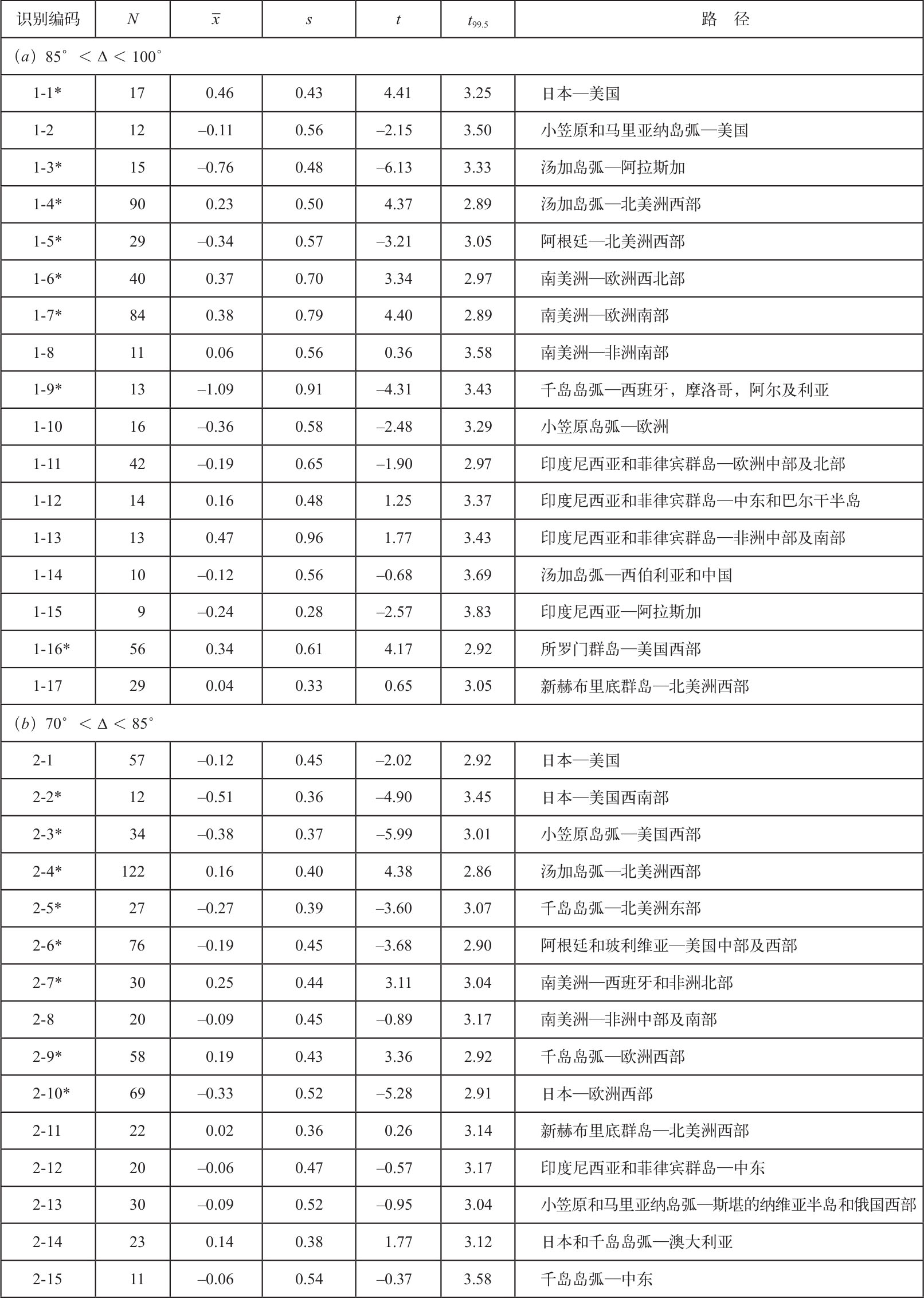
N =观测次数
=经台站校正后的平均走时残差(s)
s =残差的标准差(s)
t
=
t 99.5 =当真均值为零时,| t |的置信水平为99.5%
* 指真均值明显不为零的传播路径。
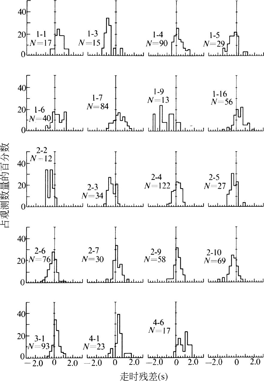
图3. 地震波沿不同路径穿过地幔的走时残差直方图(残差是相对于图1的曲线,且经过台站校正)。识别编码与表1和图4上的编码对应。 N 是观测到的地震数量。
然而,速度分布的细节无法精准测定,因为经过回折点附近几乎相同深度的不同射线传播距离相差很大。图4显示了不同路径射线束(人为限制在每条路径中心的30°)的下地幔采样区域,并指出哪些路径对应早到或晚到。这些区域往往都是真正可能出现速度异常的区域。图中一些区域重叠的地方,它们的数据也基本保持一致(例如区域1-6和1-7、2-2和2-3、4-1和4-6)。这种一致性是令人鼓舞的,因为这支持了我们的观点,即走时的异常产生于深地幔,而不是由某种系统误差所引起的。在区域1-3和1-16之间存在着显著的不一致性,但是这并不奇怪,因为走时异常实际源于何处并不确定。沿着路径1-3传播的射线穿过了区域2-2和2-3后继续向北,很可能走时异常就产生于此。图4还有一个有趣的特征,即在两个距离间隔最大的异常之间存在相关性(例如区域1-7和2-7、区域1-4和2-4、以及区域1-5和2-6),这表明深地幔的结构在垂直方向上至少在几百公里内具有一种空间“一致性”。 英文
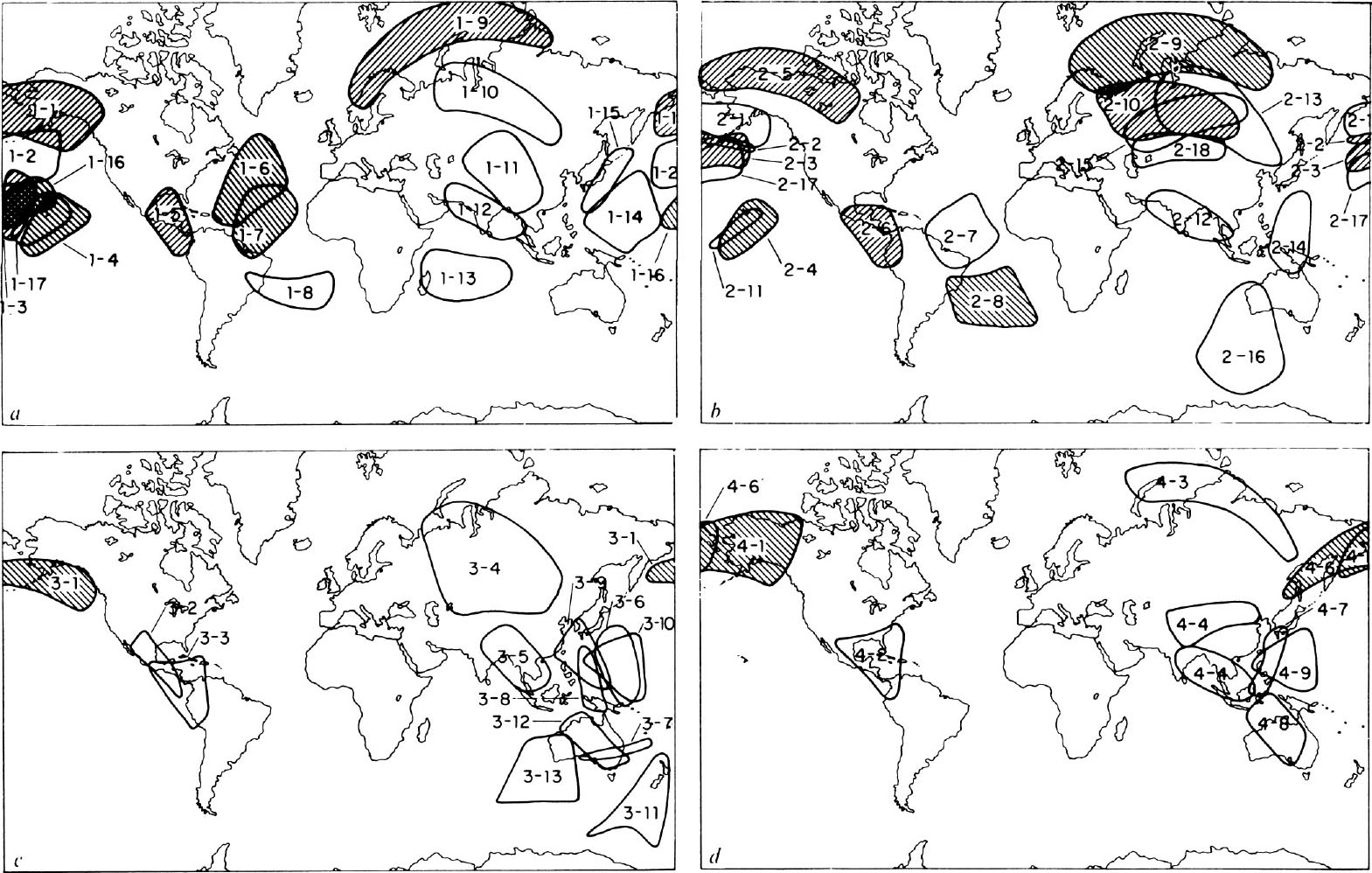
图4. 探及地幔底界的P波传播路径分区图。斜线部分表示与全部数据的平均值显著不同的区域。检测的其他区域以轮廓线表示。图中的识别编码与表1和图3的编码对应
:晚;
:早。
表1中的平均走时数据表明对于能底及2,600 km以下的射线而言,变化量约为1.5 s,而对于能底及2,000至2,600 km之间的射线来说,变化量约为0.6 s。虽然这些数据有些不确定,但是真实的走时很可能至少有1 s的变化量。地幔中实际传播速度的变化值取决于产生速度变化的区域的大小。图4中的数据显示,某些异常的尺度至少可达1,000 km或稍小,在这种情况下,传播速度至少要有1%的变化。这是一个下限,因为我们可能高估了非均质体的规模,也因为我们是在相当大的区域里测量速度平均值,很可能存在一些正负速度异常的相消效应。把有关走时的解译和d T /dΔ测量值结合起来有助于提高地幔结构细节的分辨率。 英文
深地幔的变化是否可能与威尔逊 [10] 和摩根 [11] 的地幔柱对流假说存在某种意义上的关联?对于这个问题,夏威夷群岛地区提供了极好的数据,这些数据的确显示出极其明显的横向变化:夏威夷西北部(区域2-2、2-3、可能还有1-3)的传播速度很高,而群岛附近(区域1-4、2-4和1-6)的传播速度则很低。有趣的是,戴维斯和谢泼德 [4] 提供的d T /dΔ数据也表明在夏威夷群岛附近也存在这类水平方向上的速度差异。可惜我们没能对其他设想的地幔柱进行很好的取样。区域1-13包括马斯克林群岛,但是这里的数据高度分散,不能据此得出任何结论。均具有很高传播速度的区域1-5和2-6略微靠近加拉帕戈斯群岛的东北部,因此并不清楚这里的速度异常与可能存在的地幔柱之间具有怎样的关系(假设存在一定关系的话)。如果能够获得更多穿过地幔柱的区域的地震波走时数据,或许就可以为威尔逊和摩根的假说提供有价值的证据。 英文
可能除夏威夷群岛外其他群岛的地质和构造特征没有表现出与推断的深地幔速度异常有明显的相关性。但是在较浅的深度,情况并非如此;位于千岛岛弧和阿留申岛弧下方的区域3-1、4-1和4-6,似乎都有低速异常。在这个深度上,经过充分的采样后唯一例外的一个岛弧位于中美洲下方(区域4-2),这里地震波到达得早些(虽然这些时间在99.5%的置信水平上不显著)。因此,这些数据表明在超过1,000 km的地下深处,较低的传播速度可能是岛弧的特征。 英文
这里引述的数据并不能证明在2,000 km以下的传播速度变化与地球重力异常或大地水准面高程之间有任何相关性。在较浅的深度上这种相关性确实存在,但这仅仅是地震波在千岛群岛和阿留申群岛下方低速传播的另一种表现,因为岛弧凹面一侧通常是自由空气重力正异常显著的地方。 英文
然而,这些结果与亚历山大和菲尼 [5] 的研究成果并不能进行直接比较。因为他们在北大西洋发现的异常区比我们采样的相应区域要偏东。另外,我们测量走时的方法提供了一个区域内平均传播速度的量度,而地核衍射波的情况却依赖于诸如下地幔的速度梯度等属性。对于地核盲区内传播速度的进一步研究将是下地幔走时和d T /dΔ的研究一个有益的补充。 英文
感谢戴维·戴维斯博士和纳菲·托克瑟兹博士给我们提出的建设性意见。本项研究由国防部高级研究计划局资助完成。 英文
(张效良 翻译;张忠杰 审稿)