
下载掌阅APP,畅读海量书库
立即打开


Throughout this paper,
 denote the real numbers, the complex numbers, the integers and the natural numbers respectively.We denote by
X
a real or complex Banach space,
H
a complex separable infinite dimensinal Hilbert space. Let
B
(
X
)(or
B
(
H
)) denote the algebra of all bounded linear operators on
X
(or
H
). Let
denote the real numbers, the complex numbers, the integers and the natural numbers respectively.We denote by
X
a real or complex Banach space,
H
a complex separable infinite dimensinal Hilbert space. Let
B
(
X
)(or
B
(
H
)) denote the algebra of all bounded linear operators on
X
(or
H
). Let
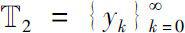
 always denote a times scales which is defined asan arbitrary nonempty closed subset of
 .
.
The theory of time scales was introduced by Hilger in his 1988 PhD dissertation
[51]
. The calculus of time scales unifies and extends the fields of discrete and continuous calculus.The delta derivative defined by Hilger
[
51
,
52
]
is equal to
f
' (the usual derivative) if
 , and it is equal to △
f
(the usual forward difference) if
, and it is equal to △
f
(the usual forward difference) if
 . So the study of dynamical equations on time scales allows a simultaneous treatment of differential and difference equations. And this field has attracted many researchers' attention
[
23
,
26
,
18
,
79
,
20
]
. In 2002, Atici and Guseinov
[9]
defined the nabla derivative by replacing the forward jump operator
σ
by backward jump operator
ρ
and researched the ▽dynamical equations on time scales.
. So the study of dynamical equations on time scales allows a simultaneous treatment of differential and difference equations. And this field has attracted many researchers' attention
[
23
,
26
,
18
,
79
,
20
]
. In 2002, Atici and Guseinov
[9]
defined the nabla derivative by replacing the forward jump operator
σ
by backward jump operator
ρ
and researched the ▽dynamical equations on time scales.
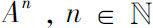
It is well known that linear systems of differential or difference equations are applied to many fields, such as mechanic systems, electric circuit and biological systems [ 23 , 79 , 10 ] . So it is meaningful to research the linear dynamical systems on time scales both in theory and applications.
For linear dynamical equations on time scales, we mainly consider the explicit formula of solutions in matrix algebra and Banach algebra, and explor the existence and uniqueness of solutions in Banach space.
Let us consider a linear system
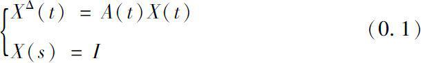
where
A
(·),
X
(·)are functions from a time scale
to
M
m
.
In the case that
 or
or
 and
A
(·)=
A
, the study of the explicit constructions of solutions to equation (0.1) has attracted many researchers' attention
[
88
,
65
,
78
,
49
,
5
,
83
,
92
]
. With the development of dynamical equations on time scales, some results have been obtained in calculating the solutions of equation (0.1) on general time scales.
and
A
(·)=
A
, the study of the explicit constructions of solutions to equation (0.1) has attracted many researchers' attention
[
88
,
65
,
78
,
49
,
5
,
83
,
92
]
. With the development of dynamical equations on time scales, some results have been obtained in calculating the solutions of equation (0.1) on general time scales.
In 1990, Hilger [52] defined a generalized exponential function on time scale and verified that it is the solution to the scalar form of equation (0.1) in the field of real numbers.
For matrix equation (0.1) in M m , Bohner and Peterson [23] defined the solution to equation (0.1) as the generalized matrix exponential function directily. They solved the exponential of a constant matrix on time scales by Putzer algorithm [88] . Then Harris algorithm and Leonard algorithm which were introduced firstly to calculate the matrix exponential e At were extended to calculate the exponential of a constant matrix on time scales [ 15 , 95 , 96 ] .
In 2007, Verde-Star
[92]
introduced an elementary method to solve linear matrix differential and difference equations and obtained explicit formulas for the classic exponential of a matrix
e
At
and
 .
.
In chapter two, we extend the method in paper [92] to solve system (0.1).Let us introduce the calculating algorithm and the explicit constructions of solutions to equation (0.1).
Let ω be any monic polynomial that is divisible by the minimal polynomial of A, i.e.,
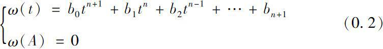
where b 0 =1.
The solution f of initial values problem

is called the dynamic solution associated with ω , where D denotes the Δderivative operator.
Define
 be the Horner polynomials of
ω
. Then the solution of equation (0.1) can be represented by the polynomial of
A
with coefficients determined by the dynamic solution associated with
ω
.
be the Horner polynomials of
ω
. Then the solution of equation (0.1) can be represented by the polynomial of
A
with coefficients determined by the dynamic solution associated with
ω
.
Theorem 0.1
Let
A
be any square matrix,
ω
be a monic polynomial as (0.2) and
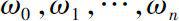 be the Horner polynomials of
ω
. If
f
(
t
) be the dynamic solution associated with
ω.
Then we have the solution of equation (0.1), i.e., the generalized matrix exponential function as follows
be the Horner polynomials of
ω
. If
f
(
t
) be the dynamic solution associated with
ω.
Then we have the solution of equation (0.1), i.e., the generalized matrix exponential function as follows
Note that the dependence on
t
of
 is completely determined by the dynamic solution
f
(
t
), which is in turn determined by the polynomial
ω
.
is completely determined by the dynamic solution
f
(
t
), which is in turn determined by the polynomial
ω
.
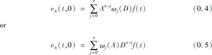
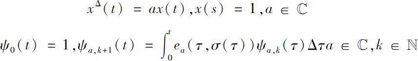
Next, let us define the basic generalized exponential polynomials on the complex plane

where
 is solution of dynamical equation
We define a commutative multiplication on
 , called the convolution product, as follows.
where
We obtain a direct construction of the dynamic solution associated with ω .
Theorem 0.2 Let ω ( t ) be as in (0.2), and

Then
 is the dynamic solution associated with
ω
.
is the dynamic solution associated with
ω
.
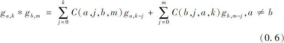
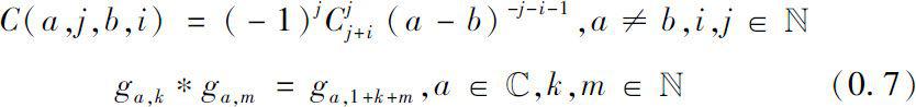
Note that we can use the recurrence relation (0.8) to compute the summands in (0.4) and (0.5). The computation of
using (0.8) is a straightforward repeated application of the convolution formula (0.6) and (0.7).
For ▽matrix dynamical equation, we can obtain the similar results as equation (0.1).
It is more difficult to obtain the constructions of solutions of time varying linear dynamic system (0.1). In chapter three we consider the explicit formula of
 with time varying function
A
(
t
). We extend the definition of generalized exponential function in the set of real numbers to the unital Banach algebra under some conditions.
with time varying function
A
(
t
). We extend the definition of generalized exponential function in the set of real numbers to the unital Banach algebra under some conditions.
Let
 denote a complex Banach algebra with unity
I
[39]
and
A
be an element in
. We define the spectrum of
A
to be the set
denote a complex Banach algebra with unity
I
[39]
and
A
be an element in
. We define the spectrum of
A
to be the set
 is not invertible in
}.
is not invertible in
}.
Let
 be rd-continuous. We define the cylinder transformation of operator value function A(t) under some spectral condition.
Let G be the single-valued and analytic branch of Logz. If the spectrum of A (·)satisfies the following condition

Then the following cylinder transformation of A (·)is reasonable.
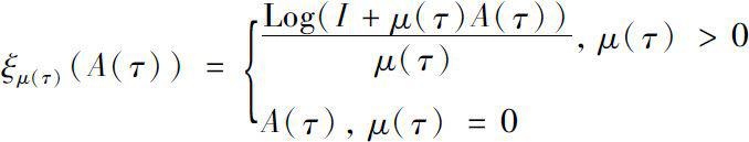
Therefore, we can define the delta exponential function on time scales in Banach algebra as follows.
Definition 0.1
Let
A
=
A
(
t
) be a rd-continuous function from a time scale
to a unital Banach algebra
(or a subalgebra of
) and satisfy the spectral conditions (
S
). Then we can define a delta exponential function of
A
(·)for
in Banach algebra as follows
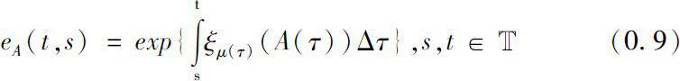
We can verify that the cylinder transformation of A (·), i.e., (0.9), is well defined by Riesz Functional Calculus and Spectral Mapping Theorem.
For
being a commutative unital Banach algebra, we obtain that, the delta exponential function defined above is just the explicit formula of the solution to system (0.1).
Theorem 0.3
Let
be a commutative (or a commutative subalgebra of) Banach algebra with unity
I
. If
A
(·)is rd-continuous and satisfies the spectral conditions (
S
), then
 is the uniqueness solution of equation (0.1).
Theorem 0.4 extends the result in scalar case to commutative Banach algebra case.
We also consider the nabla exponential function in unital Banach algebra and obtain the similar results as definition Definition 0.3 and Theorem 0.4.
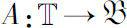
In chapter four, we consider the existence and uniqueness of global solutions to linear dynamical equations in Banach space on time scales from a new point of view.

where,

we first define a class of operators
U
as
U
:

 .
.
Then
U
is the largest class of operators which ensuring that equation (0.10) has exactly one global solution for any time scale
under some conditions.
Theorem 0.4 U is the largest one of those classes in B ( H ) which satisfy the following condition ( G ).
(
G
): “for any time scale
, if operator-valued function
A
(·):
→
U
is rd-continuous in strong operator topology, then equation (0.10) has exactly one global solution on
.”
Then we also describe the size of the class
U
on Hilbert space by characterizing its closure and interior. For
 , denote by
N
(
A
) and
R
(
A
) the kernel of
A
and the range of
A
, respectively.
A
is called a semi-Fredholm operator, if
R
(
A
) is closed and either nul
A
or nul
A
* is finite, where nul
A
: = dim
N
(
A
) andnul
A
*: = dim
N
(
A
*); in this case, ind
A
: = nul
A
– nul
A
* is called the index of
A
. In particular, if
, denote by
N
(
A
) and
R
(
A
) the kernel of
A
and the range of
A
, respectively.
A
is called a semi-Fredholm operator, if
R
(
A
) is closed and either nul
A
or nul
A
* is finite, where nul
A
: = dim
N
(
A
) andnul
A
*: = dim
N
(
A
*); in this case, ind
A
: = nul
A
– nul
A
* is called the index of
A
. In particular, if
 , then
A
is called a Fredholm operator. The Wolf spectrum
, then
A
is called a Fredholm operator. The Wolf spectrum
 of
A
is defined by
of
A
is defined by
 is not semi-Fredholm}.
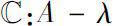
 is called the semi-Fredholm domain of
A
. For
is called the semi-Fredholm domain of
A
. For
 , we denote
 :ind (
A
-λ)=
n
}. Also, we denote
:ind (
A
-λ)=
n
}. Also, we denote
 .
.
We denote by
 the closure of
U
, and
the closure of
U
, and
 the interior of
U
.
the interior of
U
.
Theorem 0.5
Let
 . Then
(i)
 if and only if for each
 either
 ;
;
(ii)
 if and only if
 .
.
It follows from Theorem 0.5 that the class
U
has interior points. Especially in matrix algebra
M
m
, one can verify that
 . Hence we can deduce that
U
is a very large class of operators.
. Hence we can deduce that
U
is a very large class of operators.
Symmetrically, we discuss the existence and uniqueness of global solutions to nabla linear dynamical equations and obtain the similar results as theorem Theorem 0.4 and Theorem 0.5.
In 2006, Bohner and Guseinov
[19]
unified and extended the concepts of classic and discrete analytic functions to a concept of analytic functions on an arbitrary time scale complex plane
 which will be called the Δ analytic functions, where
 and
and
 are arbitrary time scales.
In 2007, Sinan [63] extended the results of paper [19] to the case of the ▽analytic functions.
In chapter five, We consider the relationship between the Δ(or▽) analytic functions and the continuous analytic functions and derive the sufficient and necessary conditions for local Δ(or▽) analytic continuation in some cases. We also research the Δ(or▽) analyticity for monomial
 and obtain some results.
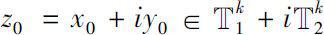
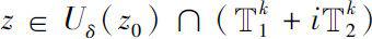
Let a function
 analytic on
 . For
. For
 , if there exists a classic analytic function
g
(
z
) on a neighborhood
, if there exists a classic analytic function
g
(
z
) on a neighborhood
 in the complex plan such that
 and
and
 for any
 . Then the function
g
(
z
) is said to be the local analytic continuation of the function
f
(
z
) at point
z
0
. If there exists locally analytic continuation of
f
(
z
) at any point
. Then the function
g
(
z
) is said to be the local analytic continuation of the function
f
(
z
) at point
z
0
. If there exists locally analytic continuation of
f
(
z
) at any point
 , then the function
f
(
z
) is said to be locally analytic continuable on
, then the function
f
(
z
) is said to be locally analytic continuable on
 .
.
we derive the sufficient and necessary conditions for local Δ analytic continuation in some cases.
Theorem 0.6
Let
 be a closed interval in
 is permitted to be unbounded interval such as

 be at most countable and without cluster point, here
 Denote
 , where
k
=1,2,3,…,
N
-1 for
N
<∞ and
k
=1,2,3,… for
N
=…∞. Supppose
, where
k
=1,2,3,…,
N
-1 for
N
<∞ and
k
=1,2,3,… for
N
=…∞. Supppose
 →
→
 be a Δ analytic function on
 and
and
 . Then there exists a unique local analytic continuation of
f
(
z
) on
. Then there exists a unique local analytic continuation of
f
(
z
) on
 if and only if the functions
 and
and
 are both real analytic function on (
a
,
b
), where
k
=1,2,3,…,
N
-1 for
N
<∞ and
k
=1,2,3,… for
N
=…∞.
are both real analytic function on (
a
,
b
), where
k
=1,2,3,…,
N
-1 for
N
<∞ and
k
=1,2,3,… for
N
=…∞.
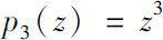
We get some results of the Δ (or▽) analyticity for monomial p n ( z )= z n , especially for n = 3, n = 4.
Theorem 0.7
Suppose
 and
and
 . Let
. Let
 be two time scales with at least one right-scattered point in
 and at least
n
right-dense points in
and at least
n
right-dense points in
 . Then there exists a point
 at which
p
n
(
z
)=
z
n
is not Δ analytic.
at which
p
n
(
z
)=
z
n
is not Δ analytic.
Theorem 0.8
Let
 be two time scales,
X
1
and
X
2
be the sets of all right-scattered points of
be two time scales,
X
1
and
X
2
be the sets of all right-scattered points of
 and
and
 separately. Then there exists at most one point in
 such that
 is Δ analytic at it. Furthermore, if
 is Δ analytic at
z
0
, then
is Δ analytic at
z
0
, then
 must be satisfied.
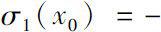
Theorem 0.9
Let
 be two time scales. If there exists right-scattered point in
and
be two time scales. If there exists right-scattered point in
and
 is a monotonic sequence converging to
y
0
. Then there exists a point
z
0
in
is a monotonic sequence converging to
y
0
. Then there exists a point
z
0
in
 such that
 is not Δ analytic at
z
0
.
is not Δ analytic at
z
0
.
We also obtain the parallel results of Δ analytic functions for ▽analytic functions on time scales.
Key words: time scales, linear dynamical system, exponential function, Banach algebra, analytic function